CNN from Scratch with pure Mathematical Intuition

Hi all,

I hope you’re equally excited as I am to embark on this journey of unraveling CNNs from the ground up. Today, we’re diving deep into the heart of convolutional neural networks, armed with nothing but our mathematical intuition. What you all need is a flavour of Linear Algebra (how matrix operations are performed), Calculus and a little focus to read and understand this article. You can trust me, I’ll not let you feel bored till the end of article. Without a further due, let’s start!

In this article, we will cover following modules (this is basically the content part we will be looking to):

1. Convolution Operation
2. Convolutional Layer
3. Reshape Layer
4. Binary Cross Entropy Loss
5. Sigmoid Activation
6. Solving MNIST

Feeling overwhelmed while looking the content above? Don’t worry, just go through the article and leave the rest on me.

1. Convolution Operation

In CNN, we have two fundamental components, Input and Kernel.

Input in CNN is typically an image or a multidimensional array representing data. Kernel is basically a small matrix of weights that perform convolution operations on input data.

Pretty sure you’ve a thought here, What is convolution?? It is a sliding window operation that combines two pieces of information, input and kernel. Let’s feel this with a real intuition.

1. Imagine you’re looking at a large painting through a small magnifying glass.

• The painting is your input image.
• The magnifying glass is your kernel.

1. You systematically move the magnifying glass across the painting, focusing on small areas at a time.

• This is like sliding the kernel over the input.

1. At each position, you’re not just looking, but also analyzing what you see.

• You might be looking for specific patterns, textures, or colors. This is analogous to the mathematical operation performed by the kernel.

1. As you move, you’re creating a new “map” of what you’ve observed.

• This new map is the output of the convolution operation, often called a feature map.

This is very fundamental operation in convolution. We perform the same operation between input & kernel that will further produce the output (another matrix).

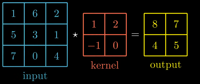
The values inside the output matrix are obtained by sliding the kernel on top of input.

Example: sliding kernel on top left of input matrix produce output as:

11 + 62 + 5 (-1) + 3*0 = 8

Likewise, we can map the kernel matrix over input and verify the output matrix.

Here’s an interesting observation in sizes of above matrices!!

Y = I - K + 1

• It refers to the output size of a convolutional operation, where: Y is the output size I is the input size K is the kernel size

But, you know? This isn’t a Convolution!!!

This operation is called Cross-Correlation.

So, What is Real Convolution?

It is basically performing same operation by rotating the kernel by 180 degrees.

i.e. new kernel matrix will be (rotating the previous matrix by 180 deg)

0	-1
2	1

We can formulate convolution as :

conv(I, K) = I * rot180(K) OR I * K = I * rot180(K), where I*K represent the Convolution!

So, the Convolution between I and K is cross-correlation between I and rotated version of K.

There are multiple ways to perform cross-correlation and hence Convolution.

What we’ve seen above is called VALID Cross-Correlation! It is basically calculating product by placing the kernel directly onto Input and start sliding when it hits the border of input.

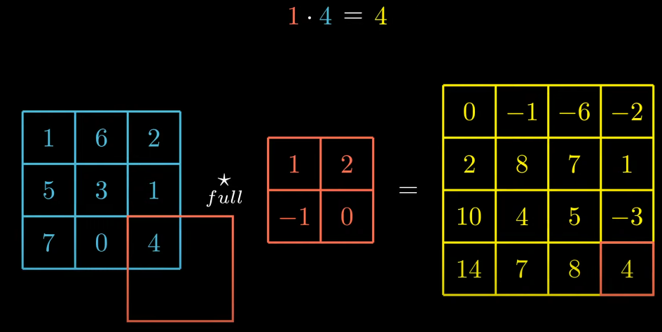
There is another way we can perform this operation called, FULL Cross-Correlation.

In this version, we calculate the product as soon as there is intersection between kernel and input matrix. Obviously, in this case size of output matrix is bigger than previous one.

One instance is shown here,

We end this module here. I assume you’ve got a basic understanding of convolution.

Let’s move forward to module 2, it is very interesting .

2. Convolutional Layer : Forward

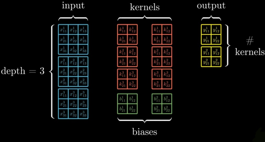
Convolutional layer takes in 3-D block of data as an input (depth=3). The layer has trainable parameters amongst the kernels (can be multiple).

Each kernel is also a 3-D block that extends full depth of input. With each kernel we associate a bias matrix that will have same shape as output matrices.

Finally, the layer will produce a 3-D block of data as output. (depth of output will be as number of kernels we have.

Let’s visualize this with a diagram.

Now the question arises, how the output is actually produced?

Let’s try to find out.

Take each matrix in first kernel and compute cross-correlation with the input data. Sum three results and add up the first bias. This will produce the first bias.

Let’s visualize this operation,

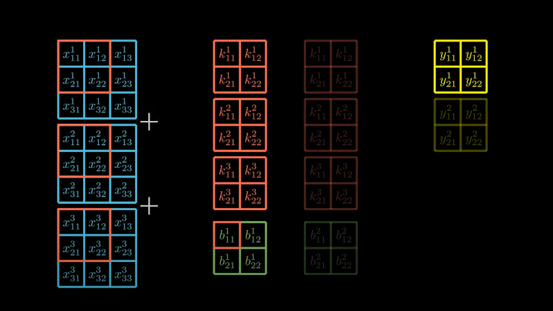
Likewise, we can perform similar operation with second kernel, input matrices and bias.

To avoid too much granularity, we can give each matrix a simple notation.

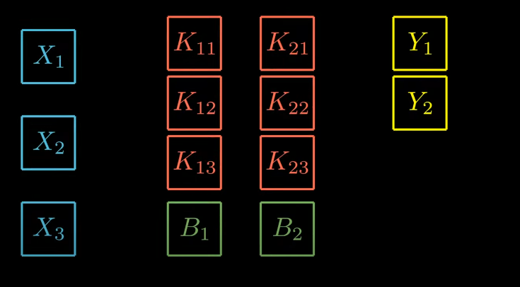
Let’s generalize the above notation with “n” input matrices and “d” as depth of output.

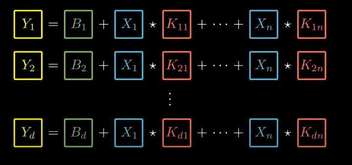
The above set of operations is known as Forward-Propagation of the convolutional layer.

We could write this more concisely using mathematical notation (Forward-Propagation Equation)

$$Yi = Bi + \sum_{j=1}^{n}Xj * Kij$$

where, i = 1 …..d

Let’s try expanding this equation (what we saw above).

This is super tempting to visualize this as a system of equations. Let’s factorize this into a single equation using matrix multiplication.

$$Y_1 = B_1 + X_1 K_{11} + \dots + X_n K_{1n}$$ $$Y_2 = B_2 + X_1 K_{21} + \dots + X_n K_{2n}$$ $$Y_d = B_d + X_1 K_{d1} + \dots + X_n K_{dn}$$

But these doesn’t work here as, these variables aren’t scalars instead matrices and “*” operation isn’t multiplication but cross-correlation.

But still, let’s pretend that we’ve an operator that does what we want. Let’s factorize these equations.

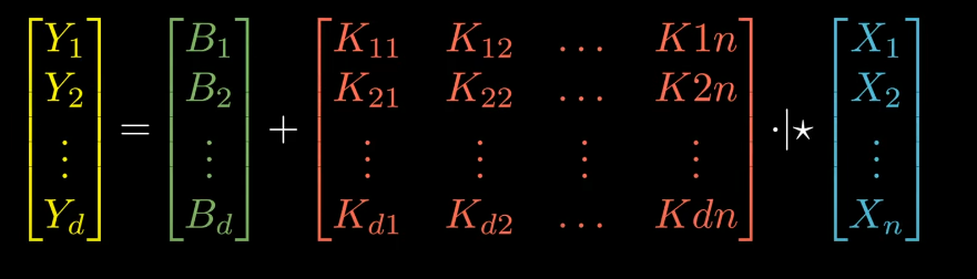
The . | * operator doesn’t exist, let’s assume it’s made up. It is basically a dot product but instead of computing multiplication between scalars then summing them up we perform cross correlation here.

We can write forward-propagation equation of the convolutional layer in a single equation.

$$Y = B + K.|* X$$

This is exact same equation that we had for the dense layer, instead of matrices of scalars we’ve matrices of matrices. Instead of regular dot product we’ve cross-correlated dot product. Actually, this is a equation of dense layer. Assume for a second, if each of the matrices is 1-D the new operator ends up being regular dot product.

So, Convolutional layer is generalization of Dense layer OR

Dense layer is particular case of Convolutional layer .

The convolutional layer inherits from the base layer that we’ve created.

Let’s write the code for forward propagation.

import numpy as np
from layer import Layer
from scipy import signal

class Convolutional(Layer):
    def __init__(self, input_shape, kernel_size, depth):
        input_depth, input_height, input_width = input_shape
        self.depth = depth
        self.input_shape = input_shape
        self.input_depth = input_depth
        self.output_shape = (depth, input_height - kernel_size + 1, input_width - kernel_size + 1)
        self.kernels_shape = (depth, input_depth, kernel_size, kernel_size)
        self.kernels = np.random.randn(*self.kernels_shape)
        self.biases = np.random.randn(*self.output_shape)

    def forward(self, input):
        self.input = input
        self.output = np.copy(self.biases)
        for i in range(self.depth):
            for j in range(self.input_depth):
                self.output[i] += signal.correlate2d(self.input[j], self.kernels[i, j], "valid")
        return self.output

    def backward(self, output_gradient, learning_rate):
        # TODO: update parameters and return input gradient
        pass

The above code is just the implementation of what we’ve seen till now. If you’re feeling overwhelmed, let me break it down with very intuitive explanation.

Imagine you have a stack of images (input). The convolutional layer is like having multiple specialized detectors (kernels) that slide over these images, looking for specific patterns.

• Each detector (kernel) is sensitive to a particular feature (like edges, textures, etc.).
• As a detector slides over the image, it produces a “heat map” of where it found its specific feature (this is the correlation operation).
• The layer has multiple sets of these detectors (depth), each creating its own set of heat maps.
• The biases allow each heat map to be adjusted up or down uniformly.

The forward method is like running all these detectors over the input images and collecting all the resulting heat maps. These heat maps (output) are then passed to the next layer of the network.

The backward method (when implemented) would adjust the detectors based on how well the network performed, making them better at finding relevant features for the task at hand.

Here, input shape is a tuple containing depth, height and width of the input.

Kernel size is the size of each matrix inside each kernel

Depth is number of kernels we want.

Biases have same shape as output (we’ve seen this before)

Convolutional Layer - Backpropagation

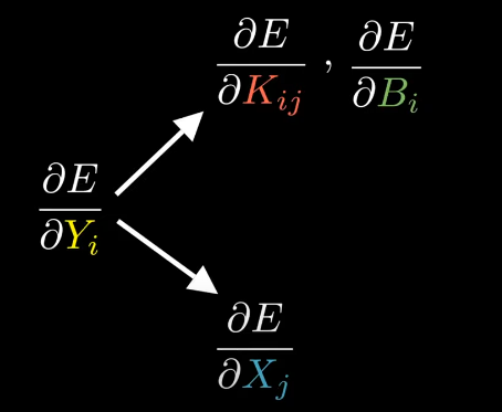
Now, in order to update the kernels and biases, we need to compute their gradients.

We are given derivative of E (error of the NN) and we need to compute two things,

a) derivative of E w.r.t trainable parameters of the layer i.e. Kernels and Biases.

b) derivative of E w.r.t input of the layer, so that the previous layer can take it as the derivative of E w.r.t to it’s own output 👇🏻

Remember the equation of forward propagation,

$$Yi = Bi + \sum_{j=1}^{n}Xj * Kij$$

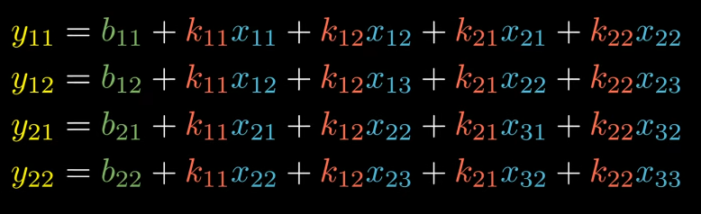
Let’s expand this again, but this time we will keep it simplified.

$$Yi = Bi + X_1 * Ki_1$$

can be shown as,

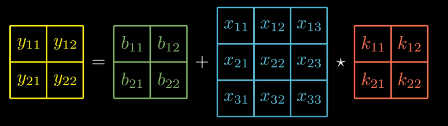
The set of equation can be shown as:

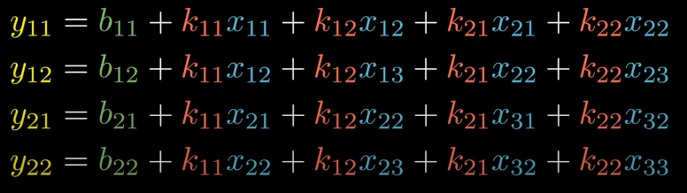
Remember , our goal is given the derivative of E w.r.t output we’ll try to compute derivative of E w.r.t kernel.

Using chain rule, we’ll get

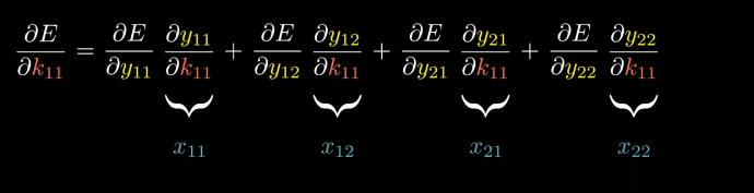
From forward propagation equation, we can see k11 appears inside every equation.

A quick question, How do I write x11 in above image?

See, if we find derivative of y11 w.r.t k11 in forward-propagation equation we’ll get x11.

Likewise, we can formulate this equation for all other 3 equations.

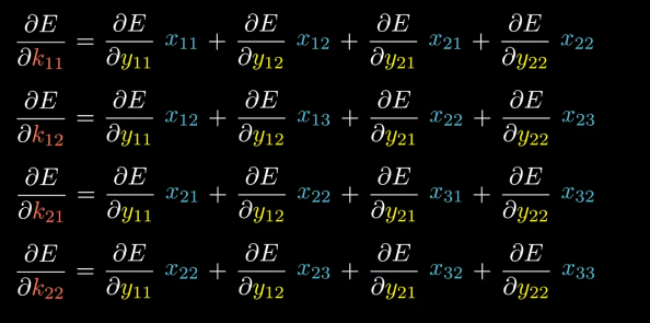
Let’s try to figure out a way to compute four derivatives above in a single formula. The first thing we can say the result is an operation between the input matrix and the matrix containing the derivatives of E w.r.t to output.

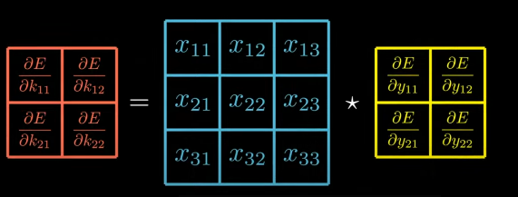
This is cross-correlation between the input matrix and the output gradient. We can write it as,

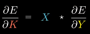
Helper Equation 1

So, we just figured out if Y = B + X * K, then we know how to compute the kernel gradient.

Remember, this is the simplified version (as we’ve talked above).

The actual equation was,

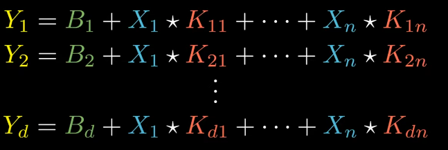
Forward Propagation Equation

We want to compute the derivative of E w.r.t K, let’s compute derivative of E w.r.t derivative of K21

It will be very tempting to use the chain rule and explain it like this:

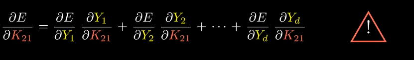
(Note: This is basic chain rule equation)

Quick question, why solving this equation is tempting or not feasible one?

Because, terms like

$$\frac{\partial Y_1}{\partial K_{21}}$$

are derivatives of matrices w.r.t other matrices and we hadn’t defined what this means.

Instead, we are going to use our helper equation 1 to solve this (we’ll take reference from forward propagation equation)

K21 appears only in the second equation i.e. equation of Y2, we can write,

$$\frac{\partial E}{\partial K_{21}} = X_1 \star \frac{\partial E}{\partial Y_2}$$

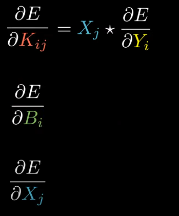
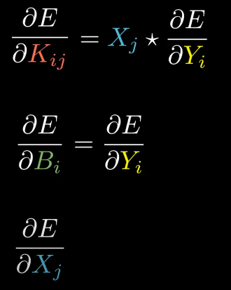
If we generalize this for any Kij, we can write:

$$\frac{\partial E}{\partial K_{ij}} = X_j \star \frac{\partial E}{\partial Y_i}$$

Theoretically challenging right!

Let’s come back to the place where we’d started this discussion!

We are interested in finding gradients (derivative of E w.r.t to derivative of kernels, bias and input matrix.)

The next step is finding Bias gradient!

We would proceed in exact same way as we did above.

Let’s directly come back to simplified version of forward propagation equation.

$$Y_i = B_i + X_1 \ast K_{i1}$$

These equations are equivalent representation of matrix form.

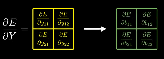
So, we are given derivative of E w.r.t output and we need to calculate derivative of E w.r.t bias.

Let’s compute derivative of E w.r.t derivative of b11.

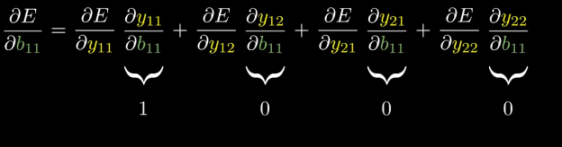
I hope you understand how we get derivatives as 1, 0, 0, 0 respectively (b11 only appears in first equation of forward propagation.)

Doing the same thing for other variables, we can clearly see that bias gradient is equal to the output gradient.

$$\frac{\partial E}{\partial b_{11}} = \frac{\partial E}{\partial y_{11}}$$ $$\frac{\partial E}{\partial b_{12}} = \frac{\partial E}{\partial y_{12}}$$

Or we can say,

$$\frac{\partial E}{\partial B} = \frac{\partial E}{\partial Y}$$

But the goal is to find derivative of E w.r.t B

Let’s start with an example, computing the derivate of E w.r.t B1 (using helper equation -2)

$$\frac{\partial E}{\partial B_{1}} = \frac{\partial E}{\partial Y_{1}}$$

We can generalize it as:

$$\frac{\partial E}{\partial B_{i}} = \frac{\partial E}{\partial Y_{i}}$$

Now, we’ve

What is left? The input gradient, in order to give it to previous layer.

This requires a good attention :)

We are given derivative of E w.r.t output and we need to calculate derivative of E w.r.t input

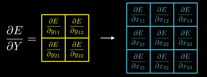
let’s compute derivative of E w.r.t derivative of x11,

![Untitled(/cnns/image22.png)

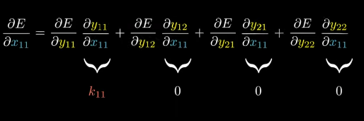
How?

x11 appears in the first equation of forward propagation and all other derivatives w.r.t x11 are 0 for other equations (w.r.t x11)

Doing this for all other x values,

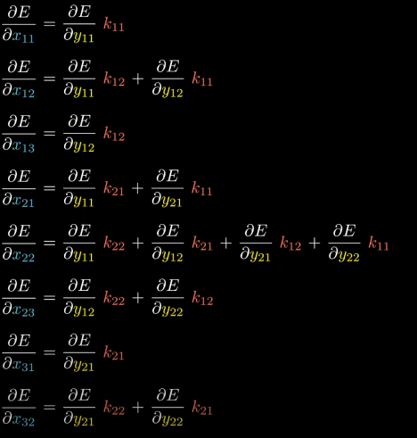
W got very unexpected! Each derivative has different number of terms added in it.

The result must be some kind of operation between the output gradient and the kernel.

Here comes the very interesting part (it was goosebumps for me when I was learning it).

The operation is a full cross correlation except that the kernel has been rotated by 180 degrees!! Remember, we’d talked about this before?

!

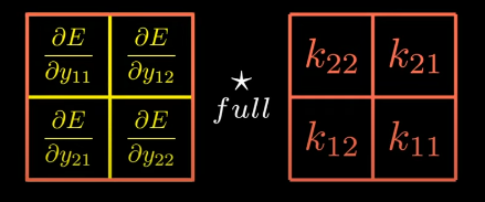
So, we’ve figured out that input gradient is equal to the output gradient fully cross-correlated with 180 degrees rotated kernel. Isn’t this the very definition of what the convolution is!!!

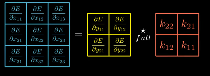
Hence, the final result is input gradient is equal to the output gradient full convolved with the kernel. Beautiful Formula!

$$\frac{\partial E}{\partial X} = \frac{\partial E}{\partial Y} \ast_{full} K$$

So, this is the simplified version.

Let’s carry out the calculation for the actual forward equation.

Remember, we need to compute derivative w.r.t to x. We’re going to start with X1 till Xj

$$\begin{aligned}\frac{\partial E}{\partial X_1} &= \frac{\partial E}{\partial Y_1} *_{full} K_{11} + \cdots + \frac{\partial E}{\partial Y_d} *_{full} K_{d1} \\[10pt] \frac{\partial E}{\partial X_j} &= \frac{\partial E}{\partial Y_1} *_{full} K_{1j} + \cdots + \frac{\partial E}{\partial Y_d} *_{full} K_{dj}\end{aligned}$$

Surprised, how did we get this. Look over the forward propagation equation, we’ve just find the derivative of all equation w.r.t Xj

If we generalize above equation, we’ll get:

$$\frac{\partial E}{\partial X_j} = \sum_{i=1}^d \frac{\partial E}{\partial Y_i} *_{full} K_{ij}, \quad j = 1 \ldots n$$

So, we finally have all three equations we needed to compute the Backward Propagation of the convolutional layer.

Now, let’s code the backward method which we’d left earlier.

import numpy as np
from layer import Layer
from scipy import signal

class Convolutional(Layer):
    def __init__(self, input_shape, kernel_size, depth):
        input_depth, input_height, input_width = input_shape
        self.depth = depth
        self.input_shape = input_shape
        self.input_depth = input_depth
        self.output_shape = (depth, input_height - kernel_size + 1, input_width - kernel_size + 1)
        self.kernels_shape = (depth, input_depth, kernel_size, kernel_size)
        self.kernels = np.random.randn(*self.kernels_shape)
        self.biases = np.random.randn(*self.output_shape)

    def forward(self, input):
        self.input = input
        self.output = np.copy(self.biases)
        for i in range(self.depth):
            for j in range(self.input_depth):
                self.output[i] += signal.correlate2d(self.input[j], self.kernels[i, j], "valid")
        return self.output
        
#--BACKWARD METHOD STARTS HERE---
    def backward(self, output_gradient, learning_rate):
        kernels_gradient = np.zeros(self.kernels_shape)
        input_gradient = np.zeros(self.input_shape)

        for i in range(self.depth):
            for j in range(self.input_depth):
                kernels_gradient[i, j] = signal.correlate2d(self.input[j], output_gradient[i], "valid")
                input_gradient[j] += signal.convolve2d(output_gradient[i], self.kernels[i, j], "full")

        self.kernels -= learning_rate * kernels_gradient
        self.biases -= learning_rate * output_gradient
        return input_gradient

The above code is just the implementation of what we’ve seen till now. If you’re feeling overwhelmed, let me break it down with very intuitive explanation.

We start by initializing empty arrays for the kernel gradient and input gradients. Next, we compute the derivative of E w.r.t Kij inside two nested for loops. We translated the mathematical formula into code mentioning the mode to be “valid” convolution. Next, we compute the input gradient. We specifically have chosen convolved2d method and mentioned mode to be “full”, which represent the full convolution. Next, we compute the bias gradient. We don’t have to calculate it since it is equal to the output gradient which is given as parameter to the backward method. The last step is to update the kernels and biases using gradient descent and return the input gradient.

You noticed something? Just 35 lines of code for entire convolutional layer.

If we want to use this layer in practice we need to implement few more things.

Our goal is solve the MNIST dataset.

It is the dataset for hand-written digits from 0 to 9, here is the sample.

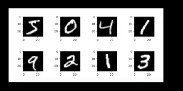
The goal is to make a neural network capable of telling what number is written on a given image.

What the code we’ve seen above isn’t optimized yet. Maybe due to compute issues, it might take a while to train a neural network on the whole dataset which contains whole 60,000 images.

For a while, let’s limit this classification to only two digits. 0 and 1.

Reshape Layer

Any guess why reshape layer is needed? Think for a while.

The output of the convolutional layer is a 3-D block. Typically, at the end of network we use dense layers which takes column vectors as input.

Therefore, we need a mechanism that reshapes the data.

Code for Reshape Layer

import numpy as np
from layer import Layer

class Reshape(Layer):
    def __init__(self, input_shape, output_shape):
        self.input_shape = input_shape
        self.output_shape = output_shape

    def forward(self, input):
        return np.reshape(input, self.output_shape)

    def backward(self, output_gradient, learning_rate):
        return np.reshape(output_gradient, self.input_shape)

The reshape layer like all the other layers inherits from the base layer class, it’s constructor takes in the shape of input and the shape of output. Forward method reshapes the input to the output.

The backward method reshapes the output to the input shape.

Binary Cross Entropy Loss

Why do we need this?

It’s because we decided to make a classification on two digits . This loss works significantly good for this task.

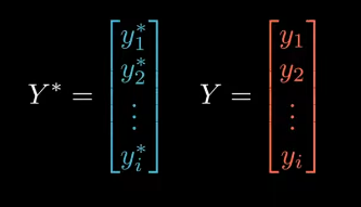
We’re given desired output of the neural network, each of the values inside the vector must either be 0 or 1. (Binary Classification). (Y)*

Then we’re given actual output of NN. (Y)

The Binary Cross Entropy is defined as:

$$E = -\frac{1}{n} \sum_{i=1}^n y_i^* \log(y_i) + (1 - y_i^*) \log(1 - y_i)$$

The goal is compute the derivative of E w.r.t output which is what we give to the backward method of the last layer of NN.

$$\frac{\partial E}{\partial Y} = [\frac{\partial E}{\partial y_1} , \frac{\partial E}{\partial y_2}, . . ....\frac{\partial E}{\partial y_i}]$$

Let’s see the derivative w.r.t y1

$$\begin{align*}\frac{\partial E}{\partial y_1} &= \frac{\partial}{\partial y_1} \left( -\frac{1}{n} \sum_{i=1}^n y_i^* \log(y_i) + (1 - y_i^*) \log(1 - y_i) \right) \\&= \frac{\partial}{\partial y_1} \left( -\frac{1}{n} (y_1^* \log(y_1) + (1 - y_1^*) \log(1 - y_1)) - \cdots - \frac{1}{n} (y_n^* \log(y_n) + (1 - y_n^*) \log(1 - y_n)) \right) \\&= \frac{\partial}{\partial y_1} \left( -\frac{1}{n} (y_1^* \log(y_1) + (1 - y_1^*) \log(1 - y_1)) \right) \\&= -\frac{1}{n} \left( \frac{y_1^*}{y_1} - \frac{1 - y_1^*}{1 - y_1} \right) \\&= \frac{1}{n} \left( \frac{1 - y_1^*}{1 - y_1} - \frac{y_1^*}{y_1} \right)\end{align*}$$

If we generalize, we’ll get

$$\frac{\partial E}{\partial y_i} = \frac{1}{n} \left( \frac{1 - y_i^*}{1 - y_i} - \frac{y_i^*}{y_i} \right)$$

So, we’ve two formulas. One Entropy, E and other the generalised equation above. We can implement them inside two separate functions.

import numpy as np

def binary_cross_entropy(y_true, y_pred):
    return -np.mean(y_true * np.log(y_pred) + (1 - y_true) * np.log(1 - y_pred))

def binary_cross_entropy_prime(y_true, y_pred):
    return ((1 - y_true) / (1 - y_pred) - y_true / y_pred) / np.size(y_true)

Note that y_true and y_pred aren’t scalars but vectors.

Sigmoid Activation

The binary cross entropy uses the logarithm function and the logarithm function can’t take negative inputs. Hence, we’re going to use sigmoid activation since it’s output is bounded in between 0 and 1.

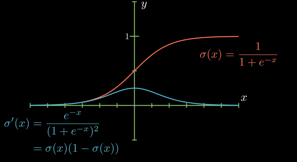
We can implement sigmoid function and it’s derivative in two separate functions.

import numpy as np
from activation import Activation

class Sigmoid(Activation):
    def __init__(self):
        def sigmoid(x):
            return 1 / (1 + np.exp(-x))

        def sigmoid_prime(x):
            s = sigmoid(x)
            return s * (1 - s)

        super().__init__(sigmoid, sigmoid_prime)

SOLVING MNIST

Now, it’s the final task to do. After publishing this blog, I’ll be solving MNIST. If you hadn’t worked on MNIST, take it as assignment to solve MNIST on your own.

I’ll attach the GitHub repository link here once I solve MNIST.

A note from my side:

Through this blog, we’ve delved deep into the mathematical foundations and implementations details of CNN from very scratch. An understanding of how neural network will ease your understanding. (I’ll add how NN works from scratch in this blog in some time).

The goal was to transform what often seems like a black box into an accessible and logical sequence of operations. I’ve taken reference from Google and YouTube for my learning before I wrote this.

Thank you for joining me on this journey. If you have any questions, feedback, or would like to share your experiences, feel free to reach out. Let’s continue to learn and innovate together!

Email : hdubey261102@gmail.com

Twitter/X: https://x.com/himanshustwts

Take care, See you soon :)