Deepseek-v3 101

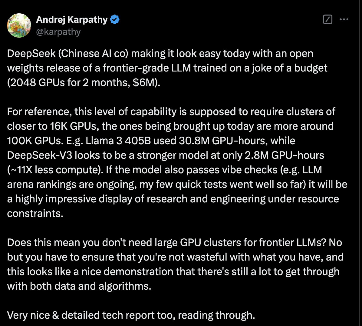
Hi! I hope you’re doing well. It’s been a long time since I’ve posted, though we are here to discuss the basic architecture of one of the best open-source models, beating Llama 3.1 405b, Qwen, and Mistral.

Deepseek v3 is the base model behind Deepseek r1.

TL;DR

• Deepseek v3 performs on par and better on many benchmarks than the big closed models by OpenAI and Anthropic.
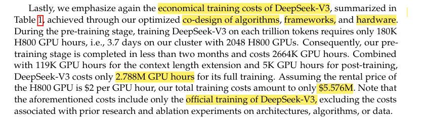
• They have incorporated Multi-Head Latent Attention, one of the crucial breakthroughs by a young undergrad in the Deepseek lab, DeepseekMoE architecture, implementing FP8 mixed precision training, and developing a custom HAI-LLM framework.
• It adapts auxiliary-loss-free-strategy for load balancing

Introduction

The architecture of DeepSeek-v3 incorporates innovative techniques like the Mixture of Experts (671B and 37B activated per token), Multi-Head Latent Attention (MHLA), and a pretraining process using 14.8T tokens. The model undergoes Supervised Fine-Tuning (SFT) and Reinforcement Learning (RL) to enhance performance. Key architectural improvements include the Load Balancing Strategy (auxiliary-loss-free) and the Multi-Token-Prediction Objective (MTP), which boosts both performance and inference speed. The model employs FP8 mixed precision during pretraining to address communication bottlenecks and integrates reasoning capabilities distilled from DeepSeek R1 series models into DeepSeek-v3.

Pre-training, context length extension, post-training-

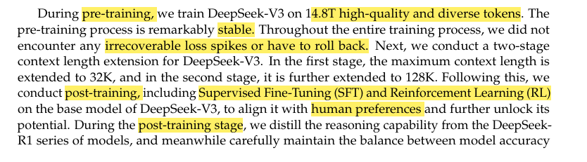
Architecture: Load Balancing Strategy - auxiliary-loss-free-strategy, Multi-Token-Prediction Objective (MTP) - model perf, inference acceleration

Pre-Training: FP8 mixed precision training framework, overcome the communication bottleneck

Post-Training: distill reasoning capabilities from the long Cot Model - Deepseek R1 series models into standard LLMs (DeepSeek-v3). pipeline incorporates the verification and reflection patterns of R1 into the model.

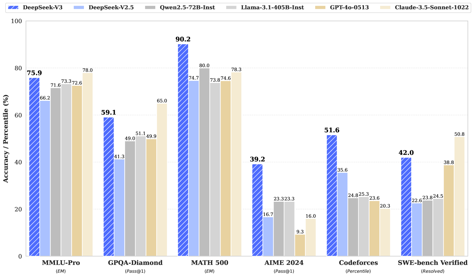
Benchmark performance of DeepSeek-V3 and its counterparts.

Architecture

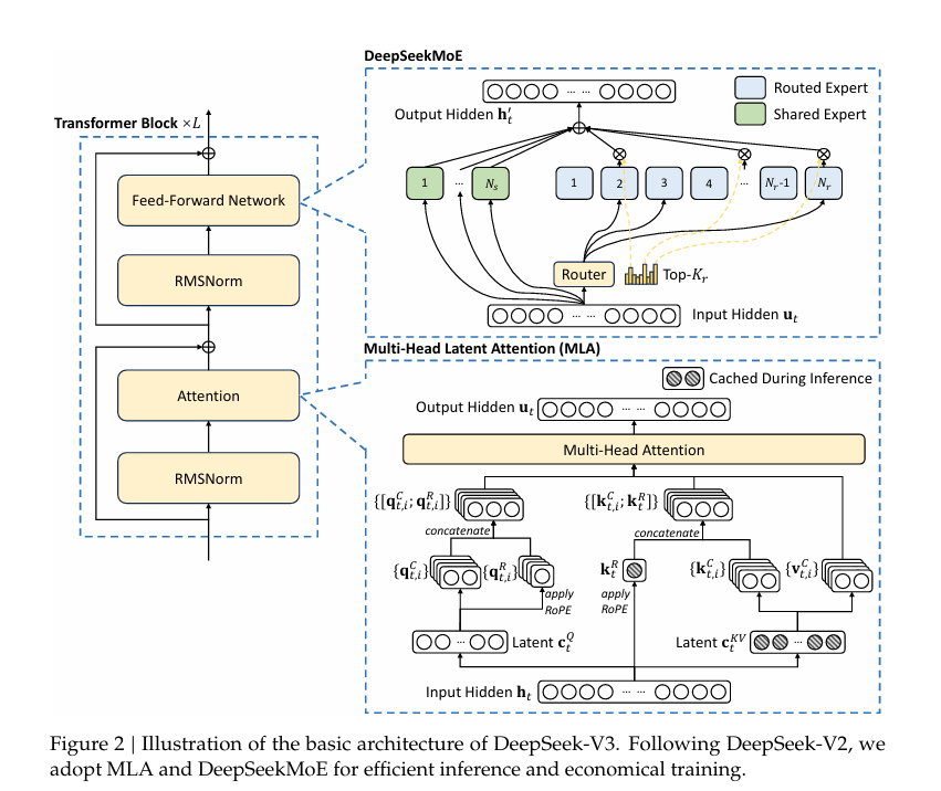
Basic Architecture of DeepSeek-v3

• Multi-Head Latent Attention
• DeepSeek MOE - Auxiliary-Loss-Free Load Balancing
• Multi-Token Prediction

In this blog, we’ll specifically focus on the newly introduced MLA and DeepseekMOE. For MTP, you can refer https://arxiv.org/abs/2404.19737

The basic Architecture of Deepseek v3 is within the Attention-Is-All-You-Need!

Multi-Head Latent Attention

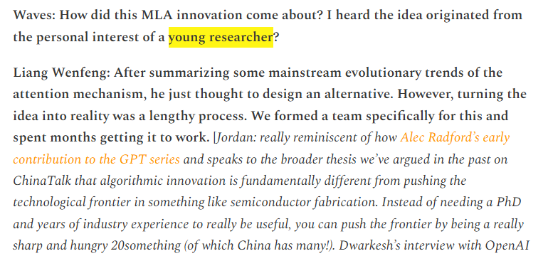
Conversation snippet with Deepseek CEO, Liang Wenfeng

• A variant of Multi-Head Attention was introduced in the DeepSeek-v2 paper.
• A major bottleneck in MHA? Heavy KV Cache that limits the inference.
• Alternatives? MQA and GQA were proposed → though they require a small amount of KV Cache the perf doesn’t match classic MHA!
• So what does MHLA solve? high perf + low KV Cache!!
• The main component of MLA → low-rank key-value joint compression

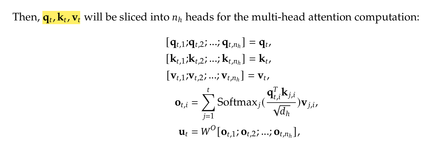
Let’s start with preliminaries of Multi-Head Attention!!

So, the standard MHA computes each attention head’s query, key, and value matrices. Why not make it more intuitive to understand?

Think of attention as a sophisticated lookup system.

BASIC BUILDING BLOCKS -

• You have an input token $h_t$ that needs to interact with other tokens
• let’s say d is the embedding dimension (how rich your token rep is)
• $n_h$ is the number of attention heads (like having multiple perspectives, X comment section?)
• $d_h$ is the dimension per head (each perspective’s detail level)

The Three core transformations would look like this -

q_t = W_Q @ h_t # What am I looking for? (Query) k_t = W_K @ h_t # What do I contain? (Key) v_t = W_V @ h_t # What’s my actual content? (Value)

Deepseek-v2 paper- page 6

Now, let’s look at memory requirements per token in MHA. This is the most interesting part, building the base for the foundations for MLA!

First, let’s understand what we need to cache!

• For each token, we need to store both Keys (K) and Values (V)
• For each token, the dimensions are:

$[K1|K2|...|Knh] = n_h * d_h elements for keys$

$V1|V2|...|Vnh] = n_h * d_h elements for values$

Total per token: $2 * n_h * d_h$ elements

sequence_length = L elements_per_token = $2 * n_h * d_h$ total_memory = sequence_length * elements_per_token = $2 * n_h * d_h * L$

As sequence length (L) grows, this linear scaling of 2nhdh elements per token becomes a significant memory constraint, so architectures like MQA, GQA, and MLA were developed to reduce this memory footprint.

Now let’s look at those architectures. We will dive deep into MLA though covering the basics of other archs.

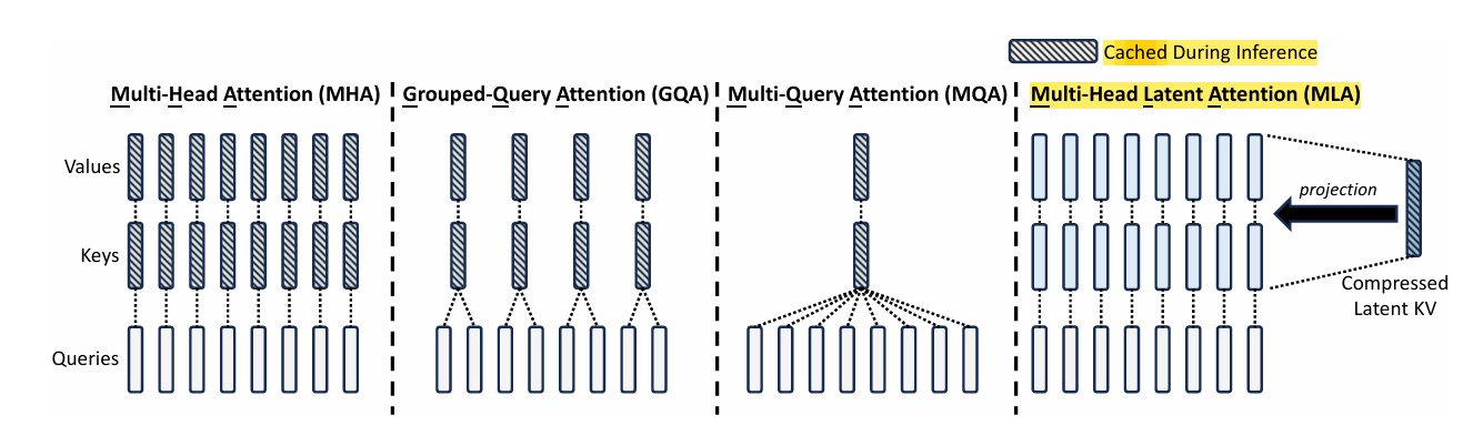
Attention architecures - Deepseek v2 paper - page 7

Standard MHA (Multi-Head Attention)

• Like having “multiple” experts looking at the same data
• Each head can focus on different aspects
• Full independence between heads

GQA (Grouped Query Attention)

• Reduces compute by sharing keys/values across groups
• GQA thinks like this: “Multiple questions looking at the same set of answers
• More efficient than full MHA

MQA (Multi-Query Attention)

• Takes sharing to the extreme: all queries share the same key/value
• Like having one reference book for all questions
• Most efficient but potentially less expressive

MLA (Multi-Head Latent Attention)

• MLA is a clever innovation that compresses key-value pairs.
• Instead of storing the full KV cache, stores the compressed version.
• Massive memory savings during inference

Low-Rank Key-Value Joint Compression

The core of MLA is the low-rank joint compression for keys and values to reduce KV cache!

• Instead of storing full key-value pairs, MLA compresses them into a shared latent space.

# Original MHA (for comparison):
key = W_K @ h_t      # Full size key
value = W_V @ h_t    # Full size value

# MLA Compression:
c_kv = W_down @ h_t  # Compressed latent vector
key = W_up_k @ c_kv  # Reconstruct key when needed
value = W_up_v @ c_kv # Reconstruct value when needed

In MLA, they incorporate a super smart idea of forming matrices via a down and up projection. The distinction is instead of storing K and V in the KV cache, we can store a small slither of C instead!

$$C = X *D, Q = X * W_q, K = C * W_{uk}, V = C * W_{uv}$$

• MLA only stores the compressed latent vector (c_kv) for each token
• Memory per token = l elements (where l is small)

# These are fixed weights of the model:
W_up_k: (n_h * d_h) × l  # One-time storage cost
W_up_v: (n_h * d_h) × l  # One-time storage cost

# What we cache PER TOKEN:
c_kv: dimension l only!   # This is what matters for scaling

# CRUCIAL DIFFERENCE

# MHA memory scaling:
tokens_memory = sequence_length * (2 * n_h * d_h)

# MLA memory scaling:
tokens_memory = sequence_length * l  # Much smaller!
model_params = 2 * (n_h * d_h * l)   # Fixed, one-time cost

So while MLA does have large projection matrices, they’re part of the model parameters (stored once) rather than per-token memory requirements.

The per-token memory (what we need to cache during inference) is just the small l-dimensional vector! This is why MLA achieves such significant memory savings during inference - you’re only storing small compressed vectors for each token instead of full key-value pairs.

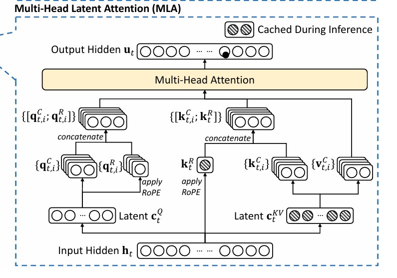
Decoupled Rotary Position Embedding (RoPE) in MLA

The RoPE problem with MLA -

Traditional RoPE applies position encoding to both K and Q

This becomes problematic with compressed KV pairs because matrix multiplication isn’t commutative

So in MLA, we can’t merge RoPE with compressed representations efficiently

Solution - Decoupled RoPE

# New approach - dECOUPLEDrOpe:
# 1. Separate position-aware queries
q_R = RoPE(W^QR @ c_q)    # Position-aware queries
k_R = RoPE(W^KR @ h_t)    # Position-aware shared key

# 2. Split into heads and concatenate
q_t,i = [q_R_1, q_R_2, ..., q_R_nh] 
k_t = [k_R_1, k_R_2]            

# 3. Concatenate for final attention
q_full = [q_t,1; q_t,2]              
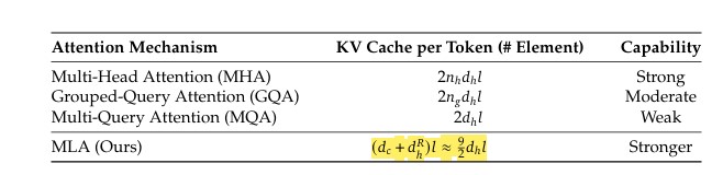
k_full = [k_t,1; k_t,2]             

Memory Requirements comparison of MHA, GQA, MQA, and MLA!

# Key parameters:
n_h = num_heads
d_h = dim_per_head
l = compression_dim
d_c = decoupled_dim

# Memory per token for each mechanism:
MHA:   2 * n_h * d_h        # Full KV storage
GQA:   2 * n_g * d_h        # Grouped KV storage
MQA:   2 * d_h              # Single KV pair
MLA:   (d_c + d_R) ≈ 4.5 * d_h # Compressed + RoPE

So MLA is equivalent to MQA with a small overhead but its performance is similar to MHA which comes out to be the best attention mechanism so far.

Insights:

• Memory efficiency close to MQA
• Performance similar to MHA
• Solves the RoPE compatibility through decoupling

A small task for you -

• How does RoPE work mathematically?

Explore, Learn, and tag me once you have the equations ready :)

Mixture of Experts (MoEs)

Imagine you’re running a large community with diverse challenges— content planning, marketing strategy, product design, etc. Instead of having everyone work on all tasks, you hire specialists: a subject expert for content, a creative designer for visuals, and so on. Whenever a task arises, the relevant expert handles it. This division of labor is more efficient and effective than having ever

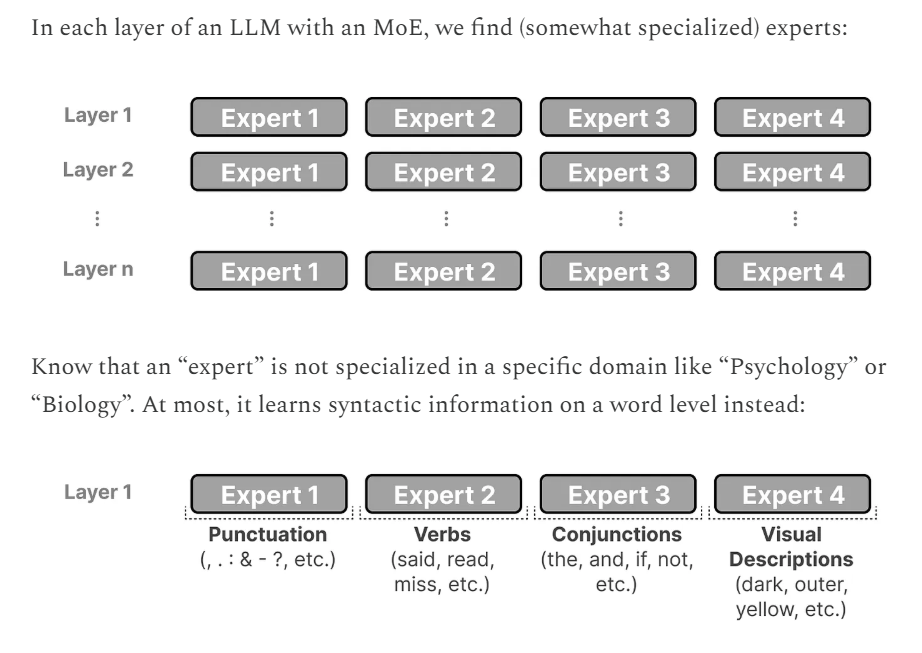
In machine learning, the Mixture of Experts (MoEs) model adopts a similar philosophy. It uses a “team” of expert neural nets, each specializing in different aspects of the data. When presented with an input, the model intelligently decides which expert(s) to involve, ensuring efficient computation and better specialization.

The expert selection process happens dynamically at each step of computation, where different experts can be activated even within the same sequence. The router network continuously evaluates which expert(s) should handle each part of the input or generation, making this a fine-grained, token-level division of labor rather than a coarse query-level split.

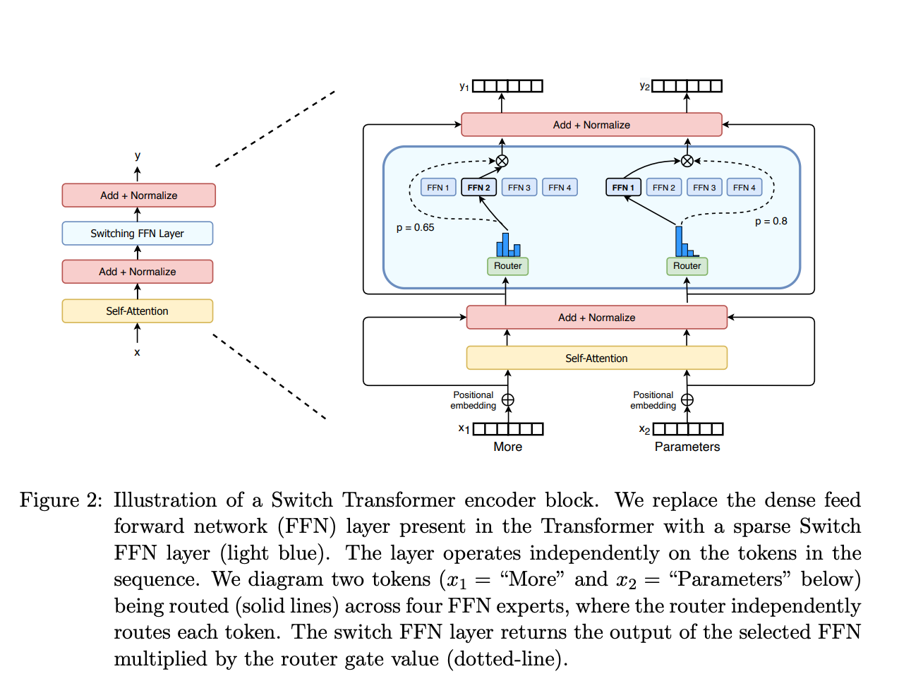
MoEs Layer from the Switch Transformer Paper

How MOEs work - A Workflow!

MOE architecture consists of the following 2 components-

• Experts
• Gating Network

Spare MOE layers are used instead of feed-forward-network (FFN) layers. These layers have a certain number of experts, and each expert is a neural net.

There is a Gating Network or Router, that determines which tokens are sent to which expert.

Workflow-

• Input Encoding - Input data is preprocessed and fed into the gating network.

• Expert Selection - The gating network evaluates the inputs and assigns weights to the experts. Typically, only a few experts are activated per input to reduce computational cost (Sparsity)

• Sparsity - It uses the idea of conditional computation (parts of the network are active on a per-example basis). While in dense models all the params are utilized for all the inputs, sparsity allows us to only run some parts of the whole system.

• Expert Contribution - Now, activated Experts process the input, and their outputs are scaled by the weights assigned by the gating network.

• Output Aggregation - Finally, the contributions from the experts are combined, usually a weighted sum, to produce the final computation.

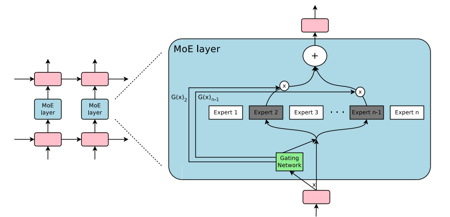
MOE layer from the Outrageously Large Neural Network paper

MOE Layers. https://newsletter.maartengrootendorst.com/p/a-visual-guide-to-mixture-of-experts

DeepSeekMoE

In section 2.1.2 of DeepSeek-v3 paper, it is mentioned that:

“Basic Architecture of DeepSeekMoE. For Feed-Forward Networks (FFNs), DeepSeek-V3 employs the DeepSeekMoE architecture (Dai et al., 2024). Compared with traditional MoE architectures like GShard (Lepikhin et al., 2021), DeepSeekMoE uses finer-grained experts and isolates some experts as shared ones.”

This ideates that DeepSeekMoE architecture builds upon the idea of Mixture of Experts (MoE) but introduces finer control and separation between shared experts and routed experts, providing better computational efficiency and performance.

Let’s understand these “experts” first.

Imagine the large community you were running. You have:

• Shared Tools (Shared Experts): These are common resources like meeting rooms or printers that everyone uses regardless of their department.

• Specialized Teams (Routed Experts): Each team is highly specialized for specific tasks, and only a subset of these teams is called upon for a given problem.

DeepSeekMOE mimics the above set of experts.

Architecture and Mathematical Details

1. Input to the Feed Forward Layer

Let $u_T$ represent the input to the FFN layer for the t-th token. This could be the output of a previous layer in the neural net. The goal is to process $u_t$ using a combination of shared experts and routed experts.

1. Output from the Feed Forward Layer

The output of the FFN layer $h'_t$ is computed as:

$$\mathbf{h}_t' = \mathbf{u}_t + \sum_{i=1}^{N_s} \text{FFN}_i^{(s)}(\mathbf{u}_t) + \sum_{i=1}^{N_r} g_{i,t} \cdot \text{FFN}_i^{(r)}(\mathbf{u}_t)$$

Here,

$N_S$: Number of shared experts

$N_r$: Number of routed experts

$\text{FFN}_i^{(s)}(\mathbf{u}_t)$: The $i_{th}$ shared expert processes the input $u_t$

$\text{FFN}_i^{(r)}(\mathbf{u}_t)$: The $i_{th}$ routed expert processes $u_t$ , but its output is scaled by gating weight

1. Gating Weights for Routed Experts

The gating weight $g_{i,t}$ for the $i-th$ routed expert is computed as

$$g_{i,t} = \frac{g_{i,t}'}{\sum_{j=1}^{N_t} g_{j,t}'}$$

Here,

$g'_{i,t}$: intermediate gating score, indicating the relevance of the $i-th$routed expert for the current input.

$g_{i,t}$: normalized gating weight, ensuring that all gating weights sums to 1.

1. Intermediate Gating Score

The intermediate gating score $g'_{i,t}$ is defined as:

$$g_{i,t}' = \begin{cases} s_{i,t} & \text{if } s_{i,t} \in \text{Top}_k(\{s_{j,t}|1 \leq j \leq N_t\}, k_r) \\0 & \text{otherwise}\end{cases}$$

Here,

$s_{i,t}$: affinity score between the token $u_t$ and the routed expert $i$ computed using a sigmoid function.

$k_r$: number of routed experts to activate (sparsity constant)

$Top_k(., k_r)$: selects the top $k_r$ experts with the highest affinity scores.

Intuitively, the gating network evaluates all routed experts and assigns scores $s_{i,t}$. Only the top $k_r$ experts (the most relevant ones) are activated. This will ensure computational efficiency by activating only a small number of routed experts.

1. Affinity Score for Routed Experts

The affinity score $s_{i,t}$ is computed as:

$$s_{i,t} = Sigmoid(u_t^Te_i)$$

Here,

$e_i$: centroid vector representing the $i-th$ routed expert

$u_t^Te_i$: measures the similarity between the token input $u_t$ and the routed expert $i$

Sigmoid(.): ensures the score is between 0 and 1

Intuitively, the routed experts act like “specialists” trained to handle certain types of input. The affinity score measures how well an expert aligns with the given input.

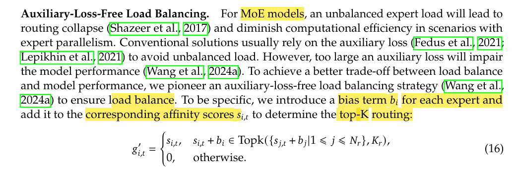
Auxillary-Loss-Free-Load-Balancing

In MoE models, each token gets routed to different experts. Without balancing, some experts get overloaded while others sit idle:

# Bad scenario:
token_distribution = {
    'expert1': 90%,  # Overloaded!
    'expert2': 5%,   # Underutilized
    'expert3': 5%    # Underutilized
}

Let’s try to understand the above Bias-Based Routing for DeepseekMoE more intuitively with an interesting analogy.

(To intuitively understand the idea behind this, just zoom the image below. This will make sense)

Think of experts as restaurants in a food delivery system:

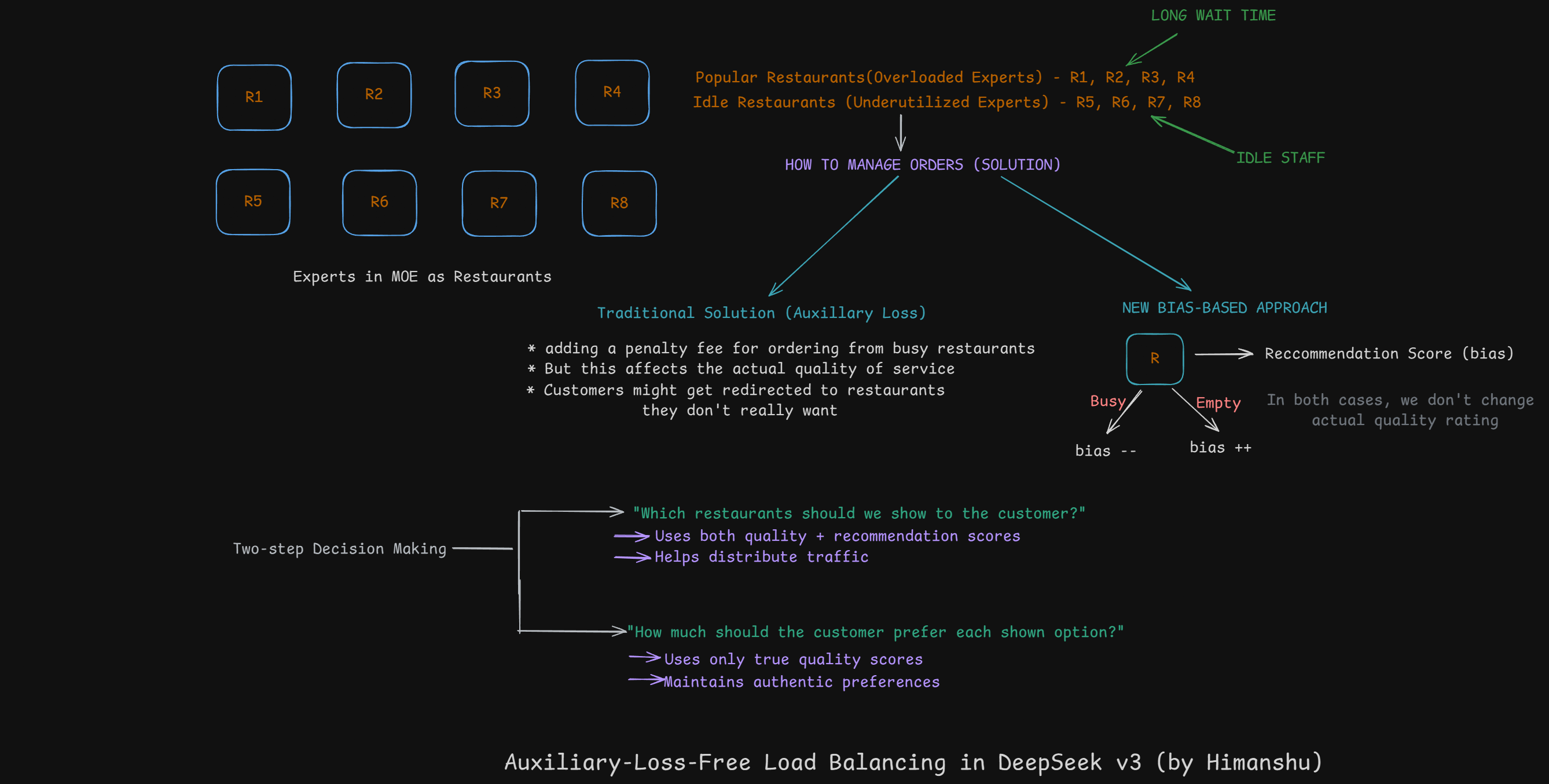
Let’s look into the bias adjustment mechanism:

Here, the bias term is only used for routing.

Routing Decision: score_for_routing = original_affinity + bias Actual Usage: gating_value = original_affinity

For each expert after each training step:
If expert is overloaded:
    bias -= γ  (make them less likely to get picked next time)
If expert is underloaded:
    bias += γ  (make them more likely to get picked next time)

The γ (gamma) parameter is like a “sensitivity knob”:

• Small γ = gentle, gradual adjustments
• Large γ = more aggressive rebalancing
• Must be tuned in to find the sweet spot

The beauty is that it maintains quality (original affinity scores) while achieving balance (through bias adjustments) - like good traffic management that doesn’t affect the destination experience.

sneak peek of Deepseek r1 architecture

References:

• Deepseek-v2

DeepSeek-V2: A Strong, Economical, and Efficient…

• Deepseek-v3

DeepSeek-V3 Technical Report

• MOE

A Visual Guide to Mixture of Experts (MoE)

• Multi-Token Prediction

Better & Faster Large Language Models via Multi-token Prediction

• Further Read: Deepseek r1

DeepSeek-R1: Incentivizing Reasoning Capability in LLMs via…

A note from my side

This is all for this blog. I hope you enjoyed reading it. Through this blog, we’ve delved deep into the concepts and mathematical foundations with intuition from the groundup.

Thank you for joining me on this journey. If you have any questions, or feedback, or would like to share your experiences, feel free to reach out. Let’s continue to learn and innovate together!

Can’t wait to publish the next one, PPO and GPQA in Deepseek r1 from first principles!

Read this blog by cneuralnets to get a general idea of Deepseek-r1:

https://trite-song-d6a.notion.site/Deepseek-R1-for-Everyone-1860af77bef3806c9db5e5c2a256577d

Take care :)