Diffusion Models - bit by bit

Hey people! Hope you’re doing well:)

I got a thought to start learning diffusion models again, I once left till learning it’s architecture.

This time I’m gonna cover from scratch, making intuitions, diving into mathematics, ideas and ending to implementation.

So this Part 1 of the series. In this part I’ve covered GANs and VAE from very scratch.

The flow of the blog will be as follows:

1. Idea behind Generative Deep Learning
2. Earlier Attempts - GANs and VAE
3. Architecture and short-comings of GANs and VAE
4. Intuition behind Diffusion Models (DDPM paper)
5. Ideation of Diffusion Models Architecture
6. Forward Pass and implementation

Idea behind Generative Deep Learning

The idea is we want to learn distribution over the data in order to generate new data

I’m assuming you all are familiar with traditional machine learning approaches where models learn to predict labels (or outputs). We never wanted to limit ourselves with only prediction based approaches, so what can be more interesting?

Here comes generative models into the picture which aims to generate new content (could be images, music, text or even realistic 3D models!)

At its core, this generative DL aims to train models to recognize the pattern or underlying structure of data.

Let’s say we want to train a model to create a scene that looks like ‘Classroom of Elite’. If we show the model enough scenic examples of the masterpiece anime, the model can start understanding patterns, textures or styles to generate scenes depending upon the context!

Earlier Attempts: GANs and VAE

So far we’ve discussed about the idea behind Generative Deep Learning. Researchers find certain approaches to bring the model into reality from ideation phase.

Evolution of GANs

In 2014, GANs (Generative Adversarial Networks) were introduced which allow generation of data by learning a distribution which mirrors that of specific set of input data (by Ian Goodfellow et al).

Let’s say we have distribution of certain images. Once the distribution is learned, data can be generated that is similar but distinct from the input data we’ve provided to the model. By ‘similar’ but ‘distinct’ from the input data I mean, it will be practically impossible from we humans to perceive the difference between input data and generated data.

The basic idea behind GAN is to have two neural networks competing against each other.

1. Generator - tries to create fake data (let’s say images) that looks like the real data.
2. Discriminator - tries to distinguish between real and fake data.

---

What does ‘Adversarial’ means in GANs?

The discriminator gets better at telling ‘fake’ from ‘real’, while generator gets better at fooling the discriminator. The ‘adversarial’ process tries to push the generator to create data that is increasingly similar to real data.

In GAN, worst case input for one of these neural nets are generated by other net. so one of the network is always trained to do as much as possible on the worst possible input.

Let’s understand with an intuition.

Suppose we have two entities: Artist (as Generator) and Art Critic (as Discriminator)

1. Artist has initially no idea and tries to create random arts. The goal is to learn how to create fake arts that are so convincing that discriminator can’t tell they’re fake. Sounds cool!
2. Critic tries to scrutinize the paintings and decide whether they are real or fake. Initially, critic can easily identify poorly generated fakes but in due course of time as generator improves, the critic must get smart to distinguish real from being fake one.

Basically, it’s a learning loop.

• generator uses the feedback from discriminator to improve, aiming to create images that are harder to distinguish from real ones.
• simultaneously, discriminator gets better at telling real from fake.

To summarise, this back-and-forth process continues.

generator → gets better at ‘fooling’ the discriminator

discriminator → sharpens it’s ability to identify fakes.

this game results in → generator producing incredibly realistic image. whoo!

---

A common use case of GAN can be ‘Image Generation’. GANs takes dataset of real images as input such as images of human faces(Ayanokoji in anime), and learn the underlying patterns. Generator model in GAN then produces entirely new, real-looking face images (Ayanokoji in real) that have never existed before. There can be many such use cases of GANs.

GANs produces outputs in high quality but most of the times they are difficult to train. This stems from adversarial setup can cause problems like vanishing gradients or mode collapse (generator keeps producing similar outputs). We will dive into architecture to understand this phenomenon.

---

It’s time to understand GAN in greater depth.

So we know GAN consist of two players (aka neural networks) : Discriminator and Generator.

The goal is to generate data that resembles the data that was in the training set. again it would be similar, but distinct.

So GANs are mostly intended to solve the task of Generative Modelling, the idea being we have a collection of training examples (could be high dimensional like images or audio waveforms).

We can ask about two things a generative model to do -

1. Density estimation

the goal is to model underlying probability distribution of the data. It helps answer “What is probability of seeing this particular data point”

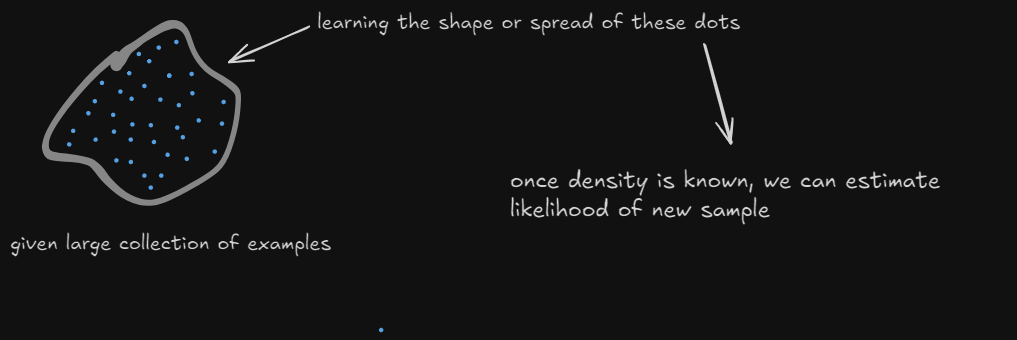
density estimation

1. Try to learn function (or program) that can generate more samples from the same training distribution.

here, the goal is to generate new data points that looks similar to the data used in training. in the analogy of artist mentioned above, after observing enough arts, the artist can create new similar paintings but aren’t exact copies as training dataset. It helps answer “Can you create new examples that look like the data I’ve trained you on?”

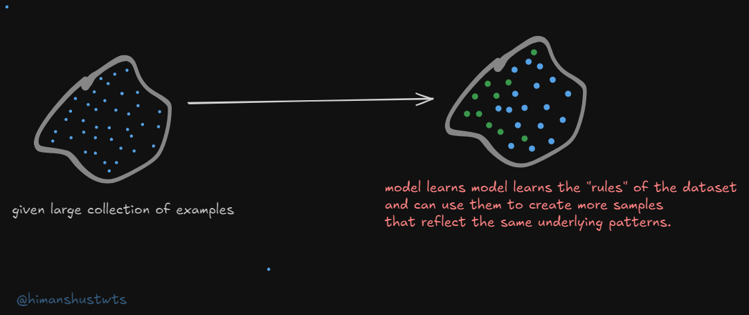
generate more samples from training distribution

The approach GAN takes to generative modelling is - two different agents playing a game against each other.

where one agent (generator network) is generating data and tries to fool the the discriminator network,

while other agent (discriminator network) tries to examine the data if it is real or fake.

Both get better and better over time and eventually generator is forced to create data that is realistic as much as possible.

---

Training Process in GAN

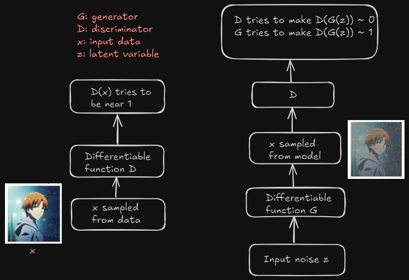
Training Process in GAN - The Architecture

Let’s breakdown the above architecture step-by-step with intuition -

1. Discriminator (Left Side)

• the goal is to distinguish between real data (actual samples from the dataset) and fake data (generated by the Generator).

How it works?

• Real data samples, represented by x, are fed into the Discriminator.
• The Discriminator is a differentiable function D(x), which outputs a value close to 1 for real data.
• The Discriminator is trained to classify real images correctly by outputting D(x) ~ 1 (i.e., “this is real”).
• If the data is real, the Discriminator’s objective is to ensure D(x) is close to 1.

1. Generator (Right side)

• the goal is to generate data that looks real in order to fool the Discriminator.

How it works?

• The Generator takes in a random noise vector z. [z is sort of randomness that allow G to output many different images instead of outputting only one realistic image]
• Using a differentiable function G(z), it produces an output (which is a fake data sample, like a fake image).
• This fake data is passed to the Discriminator (D), which will attempt to classify it as real or fake.
• The Generator’s objective is to fool the Discriminator, i.e., to produce fake data so realistic that the Discriminator outputs D(G(z)) ~ 1 (i.e., “this looks real”) and vice versa.

The Adversarial process goes like - the generator tries to generate fake data G(z) such that the discriminator classifies it as real. this means the Generator is trained to maximize D(G(z)) ≈ 1. the ****more realistic the generated data becomes, the harder it is for the discriminator to correctly identify the fake data, pushing the discriminator to improve.

---

GAME THEORY analogy to understand GAN: diving into Loss Functions

If both D and G have unlimited capabilities, the Nash Equilibrium [ a situation where no player could gain by changing their own strategy**]** corresponds to G producing perfect samples (that comes from same distribution as training data).

In other terms, the G generating fake data that is indistinguishable from real data.

The D can’t actually distinguish b/w the two sources of data and simply says every input has possibility 0.5 (for being real) and 0.5 (for being fake).

Let’s formally describe the learning process using MiniMax Game.

Loss function in a GAN captures the adversarial setup described above. It consists of two parts: one for the Discriminator and one for the Generator.

1. Discriminator’s Loss

Objective: maximize the probability of correctly classifying real data as real and fake data as fake.

it is done by maximizing real data log likelihood log D(x) (x is real data sampled from training set).

also, maximizing fake data log likelihood log(1-D(G(z)) (G(z) is the fake data generated by G from random noise ‘z’)

The discriminator loss is given as:

$$L_D = - \left( \mathbb{E}_{x \sim p_{\text{data}}(x)} [\log D(x)] + \mathbb{E}_{z \sim p_z(z)} [\log(1 - D(G(z)))] \right)$$

1. Generator’s Loss

Objective: minimize the discriminator’s ability to detect that the data it generates is fake or to fool the discriminator into thinking that G(z) is real as we saw above.

It does this by maximizing the likelihood that the Discriminator outputs 1 for the fake data G(z).

the generator loss is given as:

$$L_G = - \mathbb{E}_{z \sim p_z(z)} [\log D(G(z))]$$

So, the joint loss is a MiniMax game.

It is formulated as:

$$\min_G \max_D V(D, G) = \mathbb{E}_{x \sim p_{\text{data}}(x)} [\log D(x)] + \mathbb{E}_{z \sim p_z(z)} [\log(1 - D(G(z)))]$$

This is a zero-sum game where -

• G is minimizing the loss function (minimize the D’s ability to tell G(z) is fake)
• D is maximizing the same function (maximize D(x) for real data and minimize D(G(z)) for fake data.

---

This is pretty much about GANs and I guess you got the idea behind it’s working with an intuition. I am thinking to add a section on ‘Issues with GANs’ but without proofs that wouldn’t make much sense. I’ll add the section with more insights in few days.

If you read and got every essence of article till here, relax a bit. You really did a great job, drink some water. Try to think more, ask your self some questions - try solving those by your own.

If you find any difficulty, drop me a DM on X.

I’ll be diving deep into Variational Autoencoders now.

---

Evolution of VAE

So as we looked above, GANs rely on a game between two networks (generator and discriminator). Variational Autoencoders (VAEs) were introduced around same time but they focus on a probabilistic approach.

I’ll decode the very concept behind VAE from scratch, let’s dive deep into it.

The first question should be what are Autoencoders?

• autoencoders are trained to reconstruct input data and in the process learn reduced dimensional representation.
• the compressed features are meant to capture factors of variation in training data.

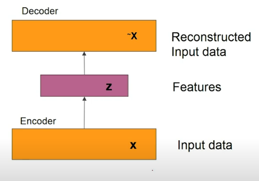
Autoencoder

---

Let’s understand the working principle of an autoencoder.

• first, the input and output sizes should be consistent enough so reconstruction loss in minimized (ex: input and output image size is 28*28)
• we pass the input data (x) to the encoder. there comes successive layers with decreasing number of hidden neurons , so we come to a layer (say it as bottleneck layer). from there again we have successively increasing number of hidden neurons in every layer till we get to the output (remember the output size is same as input size)
• this layer from which output is reconstructed is called the representation or latent space (denoted as ‘z’). though it’s difficult to impose some structure in z.

---

Let’s discuss more about Latent Space!

Imagine latent space as a low-dim space where complex data (text, image or audio) is simplified into a more manageable format. It is an abstract representation of the input data that captures its most essential features.

so, in short -

• latent space (z) is reduced dimensionality
• low-dim dimensional space which maps to an image.
• images are generated by sampling from the latent space, and mapping to an output image (draw an intuition from fig above)

why do we ideally want a latent space?

the idea is simple: we look for probabilistic/pdf for f(z) so that we can sample from it and from there we can generate images which are close to training data that we‘ve used.

---

Building mathematical foundation from Digit Generation example -

say we’ve training data : X of MNIST digits

we wish to generate digits like X (not actually present in dataset). here, we will follow a probabilistic approach and try to find P(x) of input data.

we’re trying to model that latent data.

Latent Structure

There are different strokes possible that make up the digit orientation, angle, font size, font style etc. a latent space (z) is vector off low-dim as of input data that would encode these latent structures

this ‘z’ can be sampled from the distribution, P(z).

we are looking to find a posterior distribution P(z|x).

P(z|x) → given the input dataset what would be most likely ‘z’ values that we ca have.

Idea is to map input images to a latent space using a neural network.

the latent space gives posterior distribution P(z|x) and prior distribution P(z). These both distributions can be modelled as Gaussian Distribution.

The output of given neural net has two parameters (basically the parameter of posterior distribution) → Mean(µ) and Covariance(Σ)

Now, a random sample from the latent space distribution is assumed to generate input data.

P(z|x) → x̃ (x̃ is sample from training data)

in summary, the latent space vector (a compressed representation of the input) is passed through a decoder network (another neural network), which attempts to map it back to the original input (ex: an image data).

The reconstruction output is assumed to represent the mean of a Gaussian distribution, and the difference between the reconstructed output and the original input is measured using a reconstruction loss (usually a form of mean squared error). This encourages the network to learn an effective and compact latent representation that captures key features of the data while generating realistic outputs.

---

Now, let’s come to our concerned topic:

Variational Autoencoders (VAEs)

VAE consist of three components:

1. Encoder → takes training data as input and provides parameters of Latent Space from distribution.
2. Decoder → takes samples from distribution and gives output similar (but distinct) to data in training dataset.
3. Regularized loss function → to optimise parameters of Neural Net.

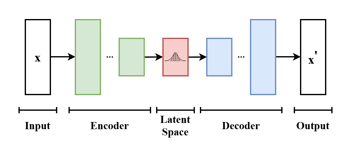
Let’s dive deep into VAE architecture and understanding it’s inner working-

So, the Encoder takes in the input data (an image, x) and maps it into latent variable ‘z’. The latent variable is not just a deterministic point but is instead sampled from a distribution.

Now, the output of encoder gives mean and covariance of Gaussian distribution over the latent space (z). Here, Θ is parameter of encoder (weights). This mean and covariance is stochastic parameter of probability distribution.

again, the idea is encoder doesn’t map the input directly to a single point in the latent space but to a distribution that captures uncertainty.

The Decoder takes latent variable from encoder, z as input (sample using mean and covariance) and reconstructs the data x̃. The goal is to generate new data that resembles the input data as closely as possible.

The output of decoder is probability distribution of the data given the latent space ‘z’. This ensures that any point sampled from latent space can be mapped back to data point in the input space, generating a new as well a realistic data. Cool!

---

Loss Function in VAEs -

This is bit complicated part in VAE, but I’ll try to breakdown it as much as I can -

Loss functions in VAEs consists of two main parts:

KL Divergence Loss (Regularization term) and Reconstruction Loss

$$-D_{KL}\left[q_{\phi}(z|x) \parallel p_{\theta}(z)\right] + \mathbb{E}_{q_{\phi}(z|x)}\left[\log(p_{\theta}(x|z))\right]$$

• The KL divergence (first term above) loss tell “how similar the two divergences are”. if they are exactly the same, we get 0 (optimum value).

This loss imposes a prior (p(z)) on the latent space to ensure the encoded representation follow a standard normal distribution → N(0,I).

also, it forces the learned latent distribution i.e. output by the encoder network to be close to standard Gaussian distribution p(z), preventing the overfitting of model.

• The Reconstruction loss aka Log-likelihood loss measures “how well the decoder can reconstruct the input data from the latent variable ‘z’”.

In case we had binary images then we would’ve chosen Binary Cross Entropy as loss function here. This loss ensures that VAE can create data similar to input.

---

What’s the idea behind using loss functions?

We want to make sure not all ‘z’ will give rise to the ‘x’ we have in our training data.

After compressing the input into the latent space, we want the decoder to reconstruct the data as closely as possible to original → handled by reconstruction loss

The KL divergence measures how much the learned distribution (produced by encoder) differs from prior distribution. It actually regularizes the latent space that keeps the model safe from overfitting.

I think, you’ve pretty much got the idea behind VAEs.

For the sake of summarising a detailed description above,

think X is a image data passed to Encoder which maps it to latent space (Z). It tries to reconstruct same X using Decoder from the Z we’ve obtained. The loss function to be optimized is done by image-by-image basis.

Visual Autoencoders (VAEs) - an Ayanokoji Story

imagine we’ve an input dataset (kiyo-art) which includes different styles of Ayanokoji paintings. the VAE process goes like:-

1. encoding (aka mapping to latent space): encoder takes each painting and compress it into latent representation, Z. here, encoder don’t represent each art with single point, but outputs a mean and variance capturing the essence of kiyo-art.
2. sampling artistic variations: from mean and variance captured above (Gaussian distribution) the model samples points in the latent space. this may generate unique rep. that maybe similar (but distinct) to any single image in kiyo-art. we can say that each point represents a new creativity on Ayanokoji.
3. decoding (aka generating new art): decoder takes this sampled latent vectors as i/p and generate new image, x̃.
4. loss calculation: VAE optimizes the model by calculating total loss for each art generated. reconstruction loss ensure the decoder to reconstruct the data as closely as possible to original. KL divergence prevents the model from generating completely unrelated arts.

Sharing some insights:

• the losses (KL divergence + reconstruction) can be minimized by backpropagation. iterative process updates parameters (Θ) of encoders and decoders.
• VAE is probabilistic approach which enables looking into new ideas by exploring variations in structured manner.

---

A note from my side

Through this blog, we’ve delved deep into the concepts and mathematical foundations with intuition from very scratch.

The goal was to transform what often seems like a black box into an accessible and logical sequence of operations. I’ve taken reference from Research Papers, blogs, YouTube tutorials to get a strong hold on my understanding of GAN and VAE and decoding the same while articulating.

Thank you for joining me on this journey. If you have any questions, feedback, or would like to share your experiences, feel free to reach out. Let’s continue to learn and innovate together!

Can’t wait to publish next one, Diffusion Models!

Take care :)

https://embed.notionlytics.com/wt/ZXlKM2IzSnJjM0JoWTJWVWNtRmphMlZ5U1dRaU9pSmhTVFZMYUdZMlkySlNiVUkxU1RreVJEbDJheUlzSW5CaFoyVkpaQ0k2SWpFd1ptSmhOR0kyWVRObVlUZ3dORFU0WkRFMlpUVTRNRE0yT0RjMU56UTNJbjA9