Transfer Learning 101

Let’s say you’ve been to Arijit’s concert and you enjoyed his songs and piano play.🎹

Now, you’re very keen to learn and play piano. However, you’ve already played instruments like violin or guitar before so you’ll not start from zero to learn piano. You already understand the rhythm, timing, and basics of music theory, so it becomes easier and faster for you to learn from your previous experiences.

Now, imagine if we could similarly teach a machine — letting it use the knowledge it already has to learn something new quickly!!

In this blog, we’ll explore the foundations and implementation of Transfer Learning from very scratch (building intuitions) covering the following topics:

• WHY Transfer Learning?
• Practical scenarios
• The Architecture behind Transfer Learning
• Mathematics behind Transfer Learning

• Perspective 1: Representation Learning
• Perspective 2: Bayesian Approach

• Hands-on Implementation

---

WHY TRANSFER LEARNING?

Let’s understand Transfer Learning in greater detail.

It is a machine learning method where a model developed for a first task is reused as the starting point for a model on a second task.

If we train a model to classify birds and cats we use the same model modified a little bit in the last layer and then use a new model to classify bees and dogs. So, it’s a very popular approach in deep learning that allows rapid generation of new models.

model used to train on birds → same model used to train on bees model used to train on cats → same model used to train on dogs

If we train the new model of bees and dogs, it can be time-consuming. That would take multiple days/weeks as well as compute.

So, if you use a pre-trained model then we typically exchange only a last layer and then don’t need to train a whole new model again.

This approach of Transfer Learning achieved good performance results and that is why it is very popular nowadays

---

PRACTICAL SCENARIOS

You may be interested what are some models we use daily that incorporate the idea of Transfer Learning. I’ve got you covered, let’s explore some of them.

1. BERT (Bidirectional Encoder Representations from Transformer)

BERT, developed by Google, introduced a model that could be pre-trained on large amounts of text and then fine-tuned for specific tasks like sentiment analysis, question answering, and more. Its bidirectional nature (understanding context from both directions in a sentence) made it particularly effective.

1. GPT (Generative Pre-trained Transformer)

OpenAI’s GPT series (GPT-2, GPT-3, GPT-4) is another landmark in transfer learning. These models are pre-trained on extensive internet text data and can be fine-tuned to perform a variety of tasks, from writing coherent essays to generating code.

1. ResNet (Residual Networks)

ResNet is an image classification model by Microsoft that won the ImageNet challenge. The architecture’s depth and transferability made it extremely effective for computer vision tasks like object detection and image segmentation, especially when fine-tuned on domain-specific image datasets.

The Architecture behind Transfer Learning

The principle behind Transfer Learning is that “knowledge gained from one task can be transferred to improve performance and efficiency on other related tasks, rather than learning each task in isolation from scratch”.

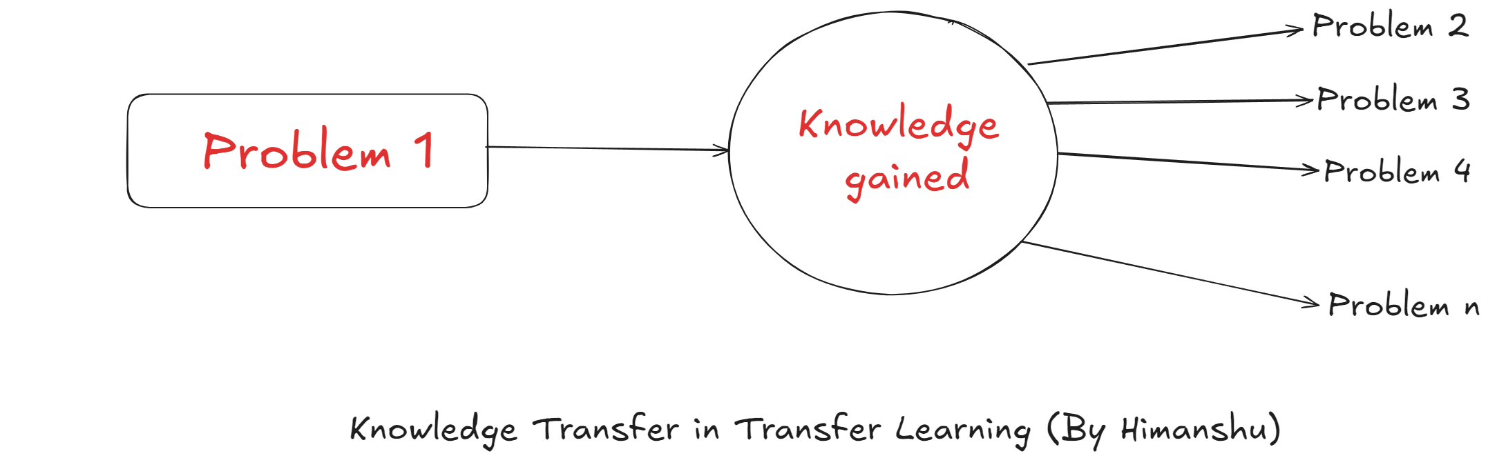
In the architecture of Transfer Learning, we have two tasks:

• Pre-trained Task
• Fine-tuning Task

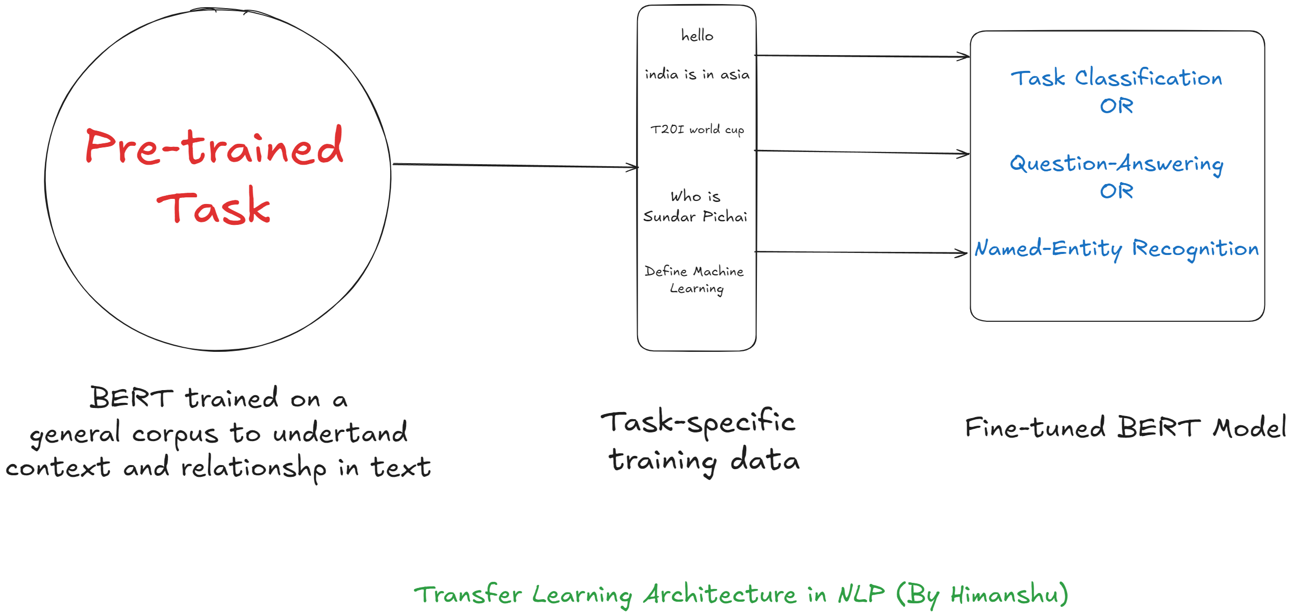
Let’s take an example of both NLP and Vision to understand this architecture.

NLP

Vision

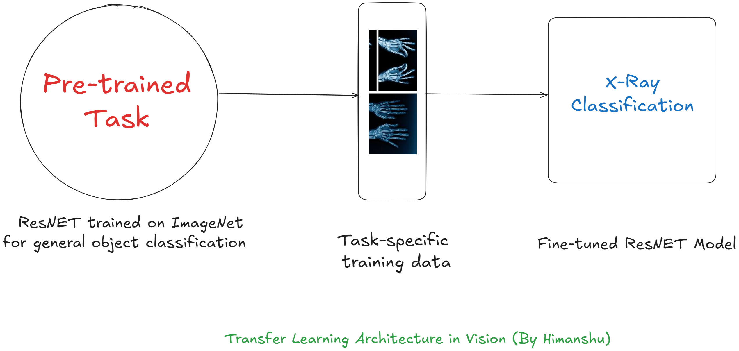
So, the idea is we extract features of the Pre-trained model and remove the last layer (or output layer) that is specific to the original task. Thereafter, we finetune the model adding a new output layer specific to our new tasks by training on our new dataset.

---

Mathematics behind Transfer Learning

As per what we’ve learned so far, Transfer Learning is fundamentally about reusing knowledge gained from a source task on a target task. Behind this idea, there is an interesting mathematics that ensures the transfer is meaningful and efficient.

Let’s go through it step by step:

Task, Domain, and Functions

• Domain(D)

A domain consists of a feature space X and a marginal probability distribution P(X).

For example, in an image classification task, X could represent pixel values, and P(X) describes how images are distributed across this feature space.

$$D = \{ X, P(X) \}$$

• Task(T)

A task consists of a label space Y and an objective function f:X→Y, which maps features to labels.

In a typical classification setting, this is the function that predicts labels given input features.

$$D = \{ Y, f(X) \}$$

Here, the goal is to transfer knowledge from a source domain Dₛ and source task Tₛ to a target domain Dₜ and target task Tₜ.

The underlying assumption is that the source and target domains or tasks share some common structure, though they aren’t identical.

Feature Learning and Reuse

Feature Extraction as Generalized Representation Learning

We know, that as we train DNNs, layers learn increasingly abstract features from the input data. The layers are divided into two categories:

• Shallow layers: (closer to the input) learn basic patterns, like edges in images or simple word representations in text
• Deeper layers: learn more task-specific features, like object parts in images or syntactic/semantic relations in text.

Intuitively, shallow layers are like noticing basic building blocks, while deeper layers put these blocks together to form a more specific, detailed understanding.

Let’s express this mathematically,

• Given input x∈X, a neural network applies a series of transformations:

$$z_1 = W_1 x + b_1, \quad a_1 = \sigma(z_1)$$ $$z_2 = W_2 a_1 + b_2, \quad a_2 = \sigma(z_2)$$ $$\vdots$$ $$y = W_n a_{n-1} + b_n$$

Wᵢ→ Weight matrics,

bᵢ→ biases,

σ is (ReLU) non-linear activation function.

Each layer i outputs an activation aᵢ, which is then passed to the next layer.

Parameter Sharing

In transfer learning, the parameters W1, W2, W3 … Wm, from earlier layers (lower-level features) are “frozen” and shared between the source task and the target task.

These parameters represent learned knowledge θs from the source domain.

• For the source task, the network learns the function:

$$fs(Xs) = f(Xs; θs)$$

θs → set of weights optimized during training on the source data Xs.

• For the target task, instead of learning a completely new set of parameters θt from scratch, transfer learning starts from θs and fine-tunes the parameters to adapt them to the target data Xt.

Loss Function and Optimization

Let’s assume the original task is trained using a loss function

Ls(θs) (something like cross-entropy for classification or mean-squared error for regression):

$$L_s(\theta_s) = \frac{1}{N_s} \sum_{i=1}^{N_t} \ell(f_s(x_i), y_i)$$

l → loss function,

Ns → number of samples in the source dataset

The optimization objective is:

$$\hat{\theta}_s = \arg \min_{\theta_s} L_s(\theta_s)$$

Now, the key idea here is that instead of training a new model ft(Xt;θt) from scratch, we use the previously learned weights θs from the source model and fine-tune them on the target task.

Fine-tuning the Model

Let’s define the new loss function for the target task:

$$L_t(\theta) = \frac{1}{N_t} \sum_{i=1}^{N_t} \ell(f_t(x_i), y_i)$$

The parameters θ are initialized from the pre-trained model, and then fine-tuned on the target task:

$$\theta_t = \arg \min_{\theta} L_t(\theta) \text{ with initialization } \theta = \hat{\theta}_s$$

Here, we initialize the network using θs, the learned parameters from the source task, instead of random initialization.

This saves computation, speeds up convergence, and helps the model achieve better performance with fewer target task examples

I hope this makes sense to you about why and how we are using the parameters from the source task :)

https://x.com/himanshustwts/status/1849156105991074155

---

Intuition from Bayesian Perspective

Let’s try to interpret transfer learning through the lens of Bayesian learning.

• Pre-training on the source task can be seen as learning a prior distribution over parameters (Prior from the source task):

$$p(\theta \mid D_s)$$

• When we transfer to the target task, we perform Bayesian updating by incorporating the target data (Posterior):

$$p(\theta \mid D_t) \propto p(D_t \mid \theta) p(\theta \mid D_s)$$

Target task data Dt updates the prior form to the posterior.

Summarising the mathematical intuition above,

Transfer learning builds on the principle of reusing previously learned parameters θs as an initialization for learning a new task θt. By sharing learned knowledge, it accelerates training, improves generalization, and reduces the data requirements for the target task.

​

---

Hands-on Implementation

Now, we will implement transfer learning from scratch using PyTorch (I’ll try explaining to you every step in this implementation).

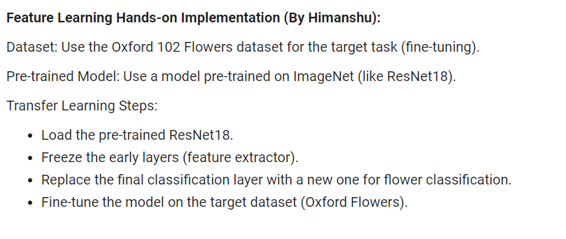
IDEA:

We will use a pre-trained model on a source task (like Imagenet) and transfer that knowledge to a target task (such as classifying flowers in the Oxford 102 Flowers dataset).

Step 1: Setting up the environment and installing the dependencies

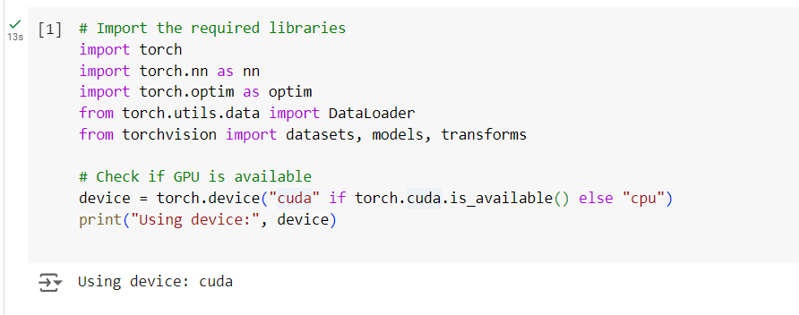
Step 2: Loading and Preprocessing the dataset

The Oxford 102 Flowers dataset consists of 102 flower categories.

Let’s load the dataset and apply necessary transformations such as resizing, cropping, and normalizing.

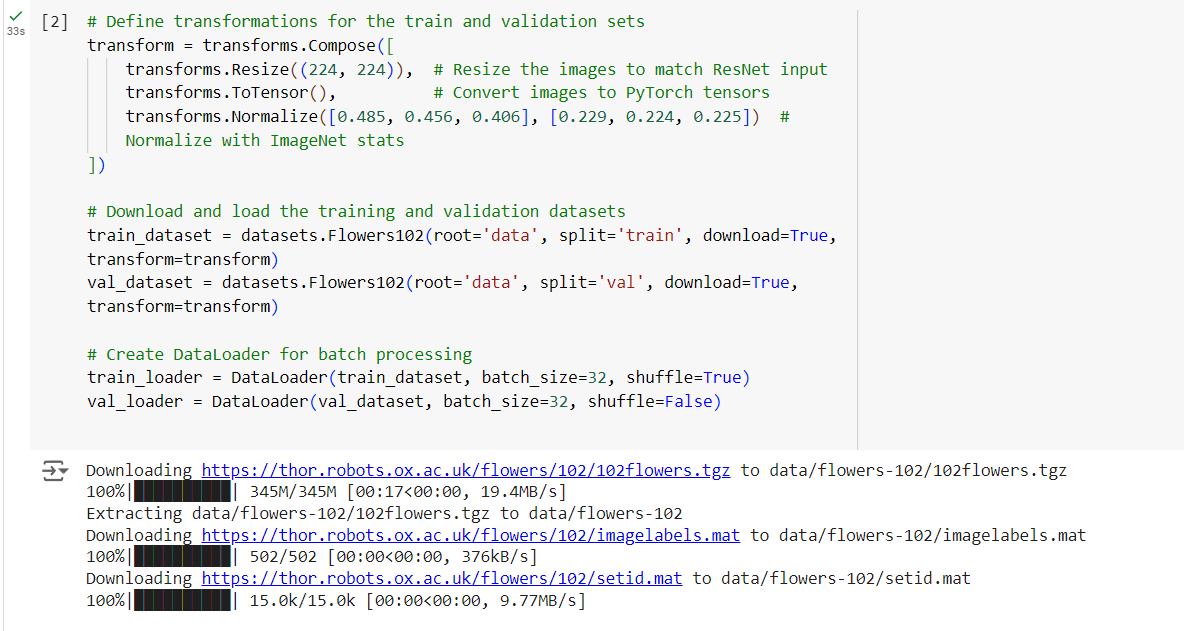
To match the ResNET’s input’s size, we resize the images to

224×224, convert them to tensors and normalize them using ImageNet’s mean and standard deviation.

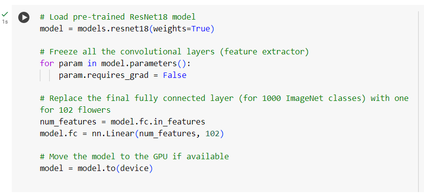
Step 3: Loading the pre-trained ResNET18 Model

Here,

• We load the pre-trained ResNet18 model.
• Freeze the layers by setting param.requires_grad = False. This prevents the early layers from being updated during backpropagation.
• Replace the final fully connected layer (model.fc) to have 102 output classes instead of 1000 (for ImageNet).

Step 4: Setting up the Loss Function and Optimizer

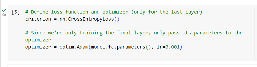
We set up the loss function (CrossEntropyLoss) and optimizer (Adam). We’ll only optimize the new fully connected layer (model.fc).

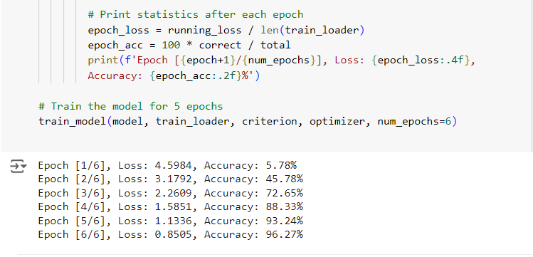
Step 5: Training the Model

We define the training loop. We will iterate over the dataset, calculate the loss, perform backpropagation, and update the model weights for the final layer.

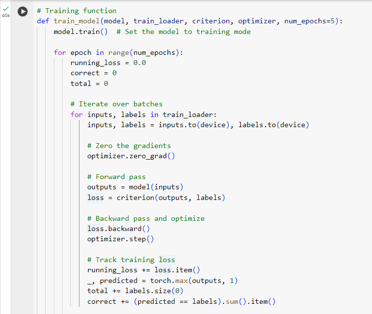
Let me share a PyTorch tip for you:

• a single training iteration in Pytorch for ‘most’ tasks requires:

forward pass calculate the loss reset current stored grad to 0 backprop loss to get new grad optimization

Let me explain what we’ve executed above:

• model.train() sets the model to training mode.

For each batch, we:

• Move the inputs and labels to the device (GPU or CPU).
• Perform a forward pass to get the predictions.
• Compute the loss using criterion.
• Perform backpropagation with loss.backward().
• Update the model’s parameters with optimizer.step().
• After each epoch (n = 6), we calculate and print the loss and accuracy.

Step 6: Evaluating the Model

After training, we evaluate the model on the validation set to check how well it has learned to classify flowers.

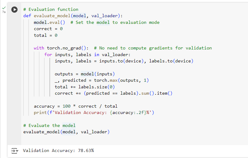
Here,

• model.eval() sets the model to evaluation mode, which disables operations like dropout.

Dropout is a technique to make models more generalizable by forcing the model to learn with redundancy, reducing overfitting, and ultimately leading to better performance on new data.

• We use torch.no_grad() to skip computing gradients, making evaluation faster. The model predicts labels on the validation set, and we compute the accuracy.

End Result: We utilized a ResNet18 model pre-trained on ImageNet to classify flowers, requiring only minimal training time and data. Validation Accuracy: 78.63%

---

Through this blog, we’ve delved deep into the concepts and mathematical foundations of transfer learning with a hands-on implementation from scratch.

Thank you for joining me on this journey. If you have any questions, or feedback, or would like to share your experiences, feel free to reach out.

Take Care :)