Understanding KL Divergence in Diffusion Generative Models and Beyond

I’ve been trying to get into rabbit holes of diffusion generative modelling from quite some time. I started drafting this blog few months back but didn’t get time to finish it up. This is some raw effort to understand KLD in diffusion generative models from ground up and beyond.

Introducing DGMs..

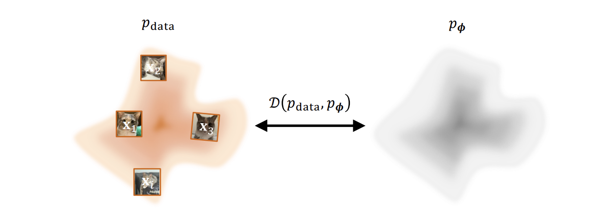
DGMs take as input a large collection of real-world examples (e.g., images,text) drawn from an unknown and complex distribution p_data and output a trained neural network that parameterizes an approximate distribution $p_{\phi}$.

Before we can learn from data, we must first decide what “learning” even means.

Consider the fundamental challenge: you observe a finite set of samples— images, sentences or molecular structures drawn from some unknown process. Your task is to build a model that captures this process well enough to generate new, plausible samples. But what does “well enough” mean? How do you measure the gap between your model and reality when reality itself is inaccessible, known only through its samples?

This is not merely a practical challenge but an epistemological one. You cannot directly compare your model’s distribution $p_{\phi}(x)$ against the true data distribution $p_{data}(x)$ because $p_{data}(x)$exists only as an abstraction.

Goal of DGM.

The sheer goal of DGM is to learn a tractable probability distribution from a finite dataset. These data points are observations assumed to be sampled from an unknown and complex true distribution $p_{data}(x)$. Since the form of $p_{data}(x)$ is unknown, we cannot draw new samples from it directly.

But what even is this form?

It refers to the mathematical expression or functional structure of the probability distribution.

When we say the “form of $p_{data}(x)$ is unknown” we mean:

1. We don’t know the equation/formula that defines the distribution
2. We don’t know what type of distribution it is (Gaussian, exponential, mixture, etc.)
3. We don’t know the parameters (mean, variance, etc.) or even how many parameters there are
4. We don’t have a closed-form mathematical expression we can write down.

And actually this is why we need deep generative models. They can learn to approximate arbitrarily complex distributions without requiring us to specify the mathematical form in advance.

So mathematically, we are trying:

$$p_{\phi^*}(\mathbf{x}) \approx p_{\text{data}}(\mathbf{x})$$

Training in DGM.

The whole field of machine learning is based on optimization. The optimization equation in this scenario is:

$$\phi^* \in \arg\min_{\phi} \mathcal{D}(p_{\text{data}}, p_{\phi})$$

where $\phi$ is trainable parameter and the training objective is to find optimal parameters $\phi^*$ (ultimately minimizing the divergence between $p_{\phi}$ and $p_{\phi^*}$

The Role of Divergence.

In information theory, a divergence is a functional D(p||q) that quantifies how one probability distribution differs from another. It is not necessarily a metric - it need not be symmetric, and it need not satisfy the triangle inequality. It is simply a principled way to assign a number to distributional difference.

The Mathematics of KL Divergence.

This essay examines KL divergence from first principles: what it measures, why it cannot be computed directly, and how its decomposition into entropy and cross-entropy enables practical optimization.

KL divergence measures how much information is lost when you approximate one distribution with another. It’s not a distance (it’s asymmetric), but rather a directed divergence.

Let’s start from what are we actually trying to do?

Step 1: The Goal

We have a dataset of images (or text, or whatever). We want to build a model that can:

1. Generate NEW samples that look like they came from the same distribution
2. Assign probabilities to data points (tell us how “likely” a sample is)

---

Step 2: The Setup

• $p_{data}(x)$: The TRUE distribution that generated our data (unknown to us)
• $p_{\phi}(x)$: Our model’s distribution (we control φ, the parameters)
• Our dataset: Just samples $\{x^{(1)}, x^{(2)}, ..., x^{(N)}\}$ drawn from $p_{data}$

We want to adjust φ so that $p_{\phi}$ becomes as close as possible to $p_{data}$.

---

Step 3: How Do We Measure “Closeness”?

This is where KL divergence comes in. KL divergence measures: “How different are two probability distributions?”

The formula is:

$$D_{\text{KL}}(p_{\text{data}} \,\|\, p_{\phi})= \int p_{\text{data}}(x)\,\log\!\left[\frac{p_{\text{data}}(x)}{p_{\phi}(x)}\right]\, dx$$

Let’s observe this a bit.

Think of it as a weighted average. For every possible x in the world ,

• Check: What’s the ratio $p_{data}(x)$ / $p_{\phi}(x)$?
• Take the log of that ratio.
• Weight it by how often x actually appears in real data.
• Sum everything up.

What Does This Ratio Mean?

$p_{data}(x)$ / $p_{\phi}(x)$ compares:

• Numerator: How likely x is in reality
• Denominator: How likely your model thinks x is

Examples:

• If $p_{data}(x)$ = 0.8 and $p_{\phi}(x)$ = 0.4, ratio = 2
  • Real data has x twice as often as your model predicts
  • Your model is underestimating this x
• If $p_{data}(x)$ = 0.2 and $p_{\phi}(x)$ = 0.8, ratio = 0.25
  • Your model thinks x is 4× more common than it actually is
  • Your model is overestimating this x

Perfect match: If $p_{data}(x)$ = $p_{\phi}(x)$ for all x, then ratio = 1, log(1) = 0, so KL = 0

---

Step 4: We can’t compute this!

Look at the formula again:

$$D_{\text{KL}}(p_{\text{data}} \,\|\, p_{\phi})= \int p_{\text{data}}(x)\,\log\!\left[\frac{p_{\text{data}}(x)}{p_{\phi}(x)}\right]\, dx$$

The issue: We don’t know what $p_{data}(x)$ is! We only have samples from it.

So we can’t evaluate:

• $p_{data}(x)$ as a function
• The integral over all possible x

---

Step 5: Let’s rewrite it!

Let’s do some algebra. Using log rules: log(a/b) = log(a) - log(b)

$$D_{\text{KL}}(p_{\text{data}} \,\|\, p_{\phi})= \int p_{\text{data}}(x)\,\bigl[\log p_{\text{data}}(x) - \log p_{\phi}(x)\bigr]\, dx$$

Split into two parts:

$$= \int p_{\text{data}}(x)\,\log p_{\text{data}}(x)\, dx \;-\; \int p_{\text{data}}(x)\,\log p_{\phi}(x)\, dx$$

Let’s name this as:

$$= [FIRST TERM] - [SECOND TERM]$$

---

Step 6: Understanding Each Term

FIRST TERM: $\int p_{\text{data}}(x)\,\log p_{\text{data}}(x)\, dx$

This is $H(p_{data})$ = the entropy of the true data distribution.

What is entropy? It measures how “random” or “spread out” the distribution is.

• High entropy: very random, unpredictable
• Low entropy: very concentrated, predictable

KEY POINT: This term has NOTHING to do with $\phi$ (our model parameters). It’s just a property of reality itself.

SECOND TERM: $\int p_{\text{data}}(x)\,\log p_{{\phi}}(x)\, dx$

This can be written as: $\mathbb{E}_{x \sim p_{\text{data}}}[\log p_{\phi}(x)]$

This is an expectation (average) over the true data distribution.

What does it mean?

• Sample x from the real data
• Evaluate: “What’s the log-probability my model assigns to x?”
• Average this over all possible x (weighted by $p_{data}$)

KEY POINT: This term DOES depend on $\phi$! We can change it by adjusting our model.

---

Step 7: The Optimization Insight

We want to:

$$\underset{\phi}{\min} \; D_{\text{KL}}(p_{\text{data}} \,\|\, p_{\phi})$$

But we just showed:

$$D_{\text{KL}}(p_{\text{data}} \,\|\, p_{\phi})= H(p_{\text{data}})- \mathbb{E}_{x \sim p_{\text{data}}}\!\left[\log p_{\phi}(x)\right]$$

There’s a magic!

$H(p_{data})$ is a constant! It doesn’t change when we change $\phi$.

So:

$$\underset{\phi}{\min} \;\bigl[\text{constant}- \mathbb{E}_{x \sim p_{\text{data}}}\!\left[\log p_{\phi}(x)\right]\bigr]$$

Is the SAME as:

$$\underset{\phi}{\max} \;\bigl[ \mathbb{E}_{x \sim p_{\text{data}}}\!\left[\log p_{\phi}(x)\right]\bigr]$$

Because minimizing (C - $f(\phi)$) is the same as maximizing $f(\phi)$.

Now our objective is:

$$\underset{\phi}{\max} \;\bigl[ \mathbb{E}_{x \sim p_{\text{data}}}\!\left[\log p_{\phi}(x)\right]\bigr]$$

This is an expectation over $p_{data}$, which we can approximate with our dataset!

With N samples $\{x^{(1)}, ..., x^{(N)}\}$:

$$\mathbb{E}_{x \sim p_{\text{data}}}\!\left[\log p_{\phi}(x)\right]\approx\frac{1}{N} \sum_{i=1}^{N} \log p_{\phi}\!\left(x^{(i)}\right)$$

This is just:

• Take each data point x^(i)
• Compute log $p_{\phi}(x^i)$ - how likely your model thinks this data point is
• Average them all

We can compute this! We don’t need to know $p_{data}(x)$ as a function anymore.

What this means in practice?

Maximum Likelihood Estimation (MLE):

Find the parameters $\phi$ that make your observed data as likely as possible under your model.

$$\phi^{*}= \underset{\phi}{\arg\max} \;\frac{1}{N} \sum_{i=1}^{N} \log p_{\phi}\!\left(x^{(i)}\right)$$

In gradient descent,

• Start with random $\phi$
• Compute the log-likelihood of your data under $p_{\phi}$
• Take gradient $\nabla_{\phi}[\log p_{\phi}(x)]$
• Update φ to increase likelihood
• Repeat

---

We’ve arrived at a remarkable equivalence: minimizing KL divergence from data is identical to maximizing likelihood of observed samples. But this equivalence conceals a deeper choice that reverberates through all of generative modeling.

Forward KL, $D_{\text{KL}}(p_{\text{data}} \,\|\, p_{\phi})$ weights errors by the true distribution. It explodes to infinity when your model assigns zero probability where data exists. This forces mode covering. Your model must explain everything it observes, even if imperfectly. It would rather be vaguely right everywhere than precisely right somewhere.

Reverse KL, $D_{\text{KL}}(p_{\phi} \,\|\, p_{data})$, weights errors by your model’s distribution. It permits ignoring data modes entirely but harshly penalizes hallucination. This induces mode seeking. Your model learns to concentrate on a subset of the data it can explain well, sacrificing coverage for precision.

Even with perfect minimization of KL divergence, we face a more fundamental problem: our samples are finite. The expectation $\mathbb{E}_{x \sim p_{\text{data}}}\!\left[\log p_{\phi}(x)\right]$ is estimated from N observations. We are not actually minimizing divergence from $p_{data}$, we are minimizing divergence from our empirical sample distribution.

The generalization question becomes: did we see enough of reality to approximate it? How many samples until the empirical distribution is close enough to the true one? This is the sample complexity of distribution learning, and it grows exponentially with dimension—the curse that modern architectures are designed to overcome.

---

Share your feedback or questions if you have any. Also if you want to discuss AI, collaborate on projects, or just chat about tech? Feel free to reach out!

X: @himanshustwts

Email: himanshu.dubey8853@gmail.com

PS: Checkout Ground Zero for deep tech podcasts with interesting folks in AI and more (coming soon).